Note
Go to the end to download the full example code.
Harmonic acoustic analysis#
This example examines a harmonic acoustic analysis that uses surface velocity to determine the steady-state response of a structure and the surrounding fluid medium to loads and excitations that vary sinusoidally with time.
Import the necessary libraries#
from pathlib import Path
from typing import TYPE_CHECKING

from PIL import Image
from ansys.mechanical.core import App
from ansys.mechanical.core.examples import delete_downloads, download_file
from matplotlib import image as mpimg
from matplotlib import pyplot as plt
from matplotlib.animation import FuncAnimation

if TYPE_CHECKING:
    import Ansys
Initialize the embedded application#
app = App(globals=globals())
print(app)
Ansys Mechanical [Ansys Mechanical Enterprise]
Product Version:252
Software build date: 06/13/2025 11:25:56
Create functions to set camera and display images#
# Set the path for the output files (images, gifs, mechdat)
output_path = Path.cwd() / "out"


def set_camera_and_display_image(
    camera,
    graphics,
    graphics_image_export_settings,
    image_output_path: Path,
    image_name: str,
    set_fit: bool = False,
) -> None:
    """Set the camera to fit the model and display the image.

    Parameters
    ----------
    camera : Ansys.ACT.Common.Graphics.MechanicalCameraWrapper
        The camera object to set the view.
    graphics : Ansys.ACT.Common.Graphics.MechanicalGraphicsWrapper
        The graphics object to export the image.
    graphics_image_export_settings : Ansys.Mechanical.Graphics.GraphicsImageExportSettings
        The settings for exporting the image.
    image_output_path : Path
        The path to save the exported image.
    image_name : str
        The name of the exported image file.
    """
    if set_fit:
        # Set the camera to fit the mesh
        camera.SetFit()
    # Export the mesh image with the specified settings
    image_path = image_output_path / image_name
    graphics.ExportImage(
        str(image_path), image_export_format, graphics_image_export_settings
    )
    # Display the exported mesh image
    display_image(image_path)


def display_image(
    image_path: str,
    pyplot_figsize_coordinates: tuple = (16, 9),
    plot_xticks: list = [],
    plot_yticks: list = [],
    plot_axis: str = "off",
) -> None:
    """Display the image with the specified parameters.

    Parameters
    ----------
    image_path : str
        The path to the image file to display.
    pyplot_figsize_coordinates : tuple
        The size of the figure in inches (width, height).
    plot_xticks : list
        The x-ticks to display on the plot.
    plot_yticks : list
        The y-ticks to display on the plot.
    plot_axis : str
        The axis visibility setting ('on' or 'off').
    """
    # Set the figure size based on the coordinates specified
    plt.figure(figsize=pyplot_figsize_coordinates)
    # Read the image from the file into an array
    plt.imshow(mpimg.imread(image_path))
    # Get or set the current tick locations and labels of the x-axis
    plt.xticks(plot_xticks)
    # Get or set the current tick locations and labels of the y-axis
    plt.yticks(plot_yticks)
    # Turn off the axis
    plt.axis(plot_axis)
    # Display the figure
    plt.show()
Configure graphics for image export#
graphics = app.Graphics
camera = graphics.Camera

# Set the camera orientation to isometric view
camera.SetSpecificViewOrientation(ViewOrientationType.Iso)

# Set the image export format to PNG and configure the export settings
image_export_format = GraphicsImageExportFormat.PNG
settings_720p = Ansys.Mechanical.Graphics.GraphicsImageExportSettings()
settings_720p.Resolution = GraphicsResolutionType.EnhancedResolution
settings_720p.Background = GraphicsBackgroundType.White
settings_720p.Width = 1280
settings_720p.Height = 720
settings_720p.CurrentGraphicsDisplay = False
camera.Rotate(180, CameraAxisType.ScreenY)
Download geometry and materials files#
# Download the geometry file from the ansys/example-data repository
geometry_path = download_file("C_GEOMETRY.agdb", "pymechanical", "embedding")
# Download the material file from the ansys/example-data repository
mat_path = download_file("Air-material.xml", "pymechanical", "embedding")
Import the geometry#
# Define the model
model = app.Model
# Add the geometry import group and set its preferences
geometry_import = model.GeometryImportGroup.AddGeometryImport()
geometry_import_format = (
Ansys.Mechanical.DataModel.Enums.GeometryImportPreference.Format.Automatic
)
geometry_import_preferences = Ansys.ACT.Mechanical.Utilities.GeometryImportPreferences()
geometry_import_preferences.ProcessNamedSelections = True
# Import the geometry file with the specified format and preferences
geometry_import.Import(
geometry_path, geometry_import_format, geometry_import_preferences
)
# Define the geometry in the model
geometry = model.Geometry
# Suppress the bodies at the specified geometry.Children indices
suppressed_indices = [0, 1, 2, 3, 4, 6, 9, 10]
for index, child in enumerate(geometry.Children):
if index in suppressed_indices:
child.Suppressed = True
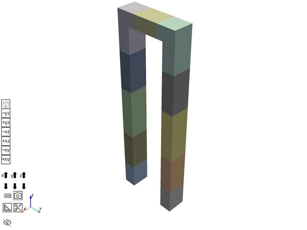
# Visualize the model in 3D
app.plot()
Store all variables necessary for analysis#
mesh = model.Mesh
named_selection = model.NamedSelections
connection = model.Connections
coordinate_systems = model.CoordinateSystems
mat = model.Materials
Set up the analysis#
# Add the harmonic acoustics analysis and unit system
model.AddHarmonicAcousticAnalysis()
app.ExtAPI.Application.ActiveUnitSystem = MechanicalUnitSystem.StandardMKS
Import and assign the materials
mat.Import(mat_path)

# Assign the material to the ``geometry.Children`` bodies that are not suppressed
for child in range(geometry.Children.Count):
    if child not in suppressed_indices:
        geometry.Children[child].Material = "Air"
Create a coordinate system
lcs1 = coordinate_systems.AddCoordinateSystem()
lcs1.OriginX = Quantity("0 [mm]")
lcs1.OriginY = Quantity("0 [mm]")
lcs1.OriginZ = Quantity("0 [mm]")
lcs1.PrimaryAxisDefineBy = CoordinateSystemAlignmentType.GlobalZ
Generate the mesh
mesh.ElementSize = Quantity("200 [mm]")
mesh.GenerateMesh()
Create named selections#
Create a function to set up named selections
def setup_named_selection(scoping_method, name):
    """Create a named selection with the specified scoping method and name.

    Parameters
    ----------
    scoping_method : GeometryDefineByType
        The scoping method for the named selection.
    name : str
        The name of the named selection.

    Returns
    -------
    Ansys.ACT.Automation.Mechanical.NamedSelection
        The created named selection.
    """
    ns = model.AddNamedSelection()
    ns.ScopingMethod = scoping_method
    ns.Name = name
    return ns
Create a function to add generation criteria to the named selection
def add_generation_criteria(
    named_selection,
    value,
    active=True,
    action=SelectionActionType.Add,
    entity_type=SelectionType.GeoFace,
    criterion=SelectionCriterionType.Size,
    operator=SelectionOperatorType.Equal,
):
    """Add generation criteria to the named selection.

    Parameters
    ----------
    named_selection : Ansys.ACT.Automation.Mechanical.NamedSelection
        The named selection to which the criteria will be added.
    value : Quantity
        The value for the criteria.
    active : bool
        Whether the criteria is active.
    action : SelectionActionType
        The action type for the criteria.
    entity_type : SelectionType
        The entity type for the criteria.
    criterion : SelectionCriterionType
        The criterion type for the criteria.
    operator : SelectionOperatorType
        The operator for the criteria.
    """
    generation_criteria = named_selection.GenerationCriteria
    criteria = Ansys.ACT.Automation.Mechanical.NamedSelectionCriterion()
    criteria.Active = active
    criteria.Action = action
    criteria.EntityType = entity_type
    criteria.Criterion = criterion
    criteria.Operator = operator
    criteria.Value = value
    generation_criteria.Add(criteria)
Add a named selection for the surface velocity and define its generation criteria
sf_velo = setup_named_selection(GeometryDefineByType.Worksheet, "sf_velo")
add_generation_criteria(sf_velo, Quantity("3e6 [mm^2]"))
add_generation_criteria(
    sf_velo,
    Quantity("15000 [mm]"),
    action=SelectionActionType.Filter,
    criterion=SelectionCriterionType.LocationZ,
)
# Activate and generate the named selection
sf_velo.Activate()
sf_velo.Generate()
Add named selections for the absorption faces and define its generation criteria
abs_face = setup_named_selection(GeometryDefineByType.Worksheet, "abs_face")
add_generation_criteria(abs_face, Quantity("1.5e6 [mm^2]"))
add_generation_criteria(
    abs_face,
    Quantity("500 [mm]"),
    action=SelectionActionType.Filter,
    criterion=SelectionCriterionType.LocationY,
)
# Activate and generate the named selection
abs_face.Activate()
abs_face.Generate()
Add named selections for the pressure faces and define its generation criteria
pres_face = setup_named_selection(GeometryDefineByType.Worksheet, "pres_face")
add_generation_criteria(pres_face, Quantity("1.5e6 [mm^2]"))
add_generation_criteria(
    pres_face,
    Quantity("4500 [mm]"),
    action=SelectionActionType.Filter,
    criterion=SelectionCriterionType.LocationY,
)
# Activate and generate the named selection
pres_face.Activate()
pres_face.Generate()
Add named selections for the acoustic region and define its generation criteria
acoustic_region = setup_named_selection(
    GeometryDefineByType.Worksheet, "acoustic_region"
)
add_generation_criteria(
    acoustic_region,
    8,
    entity_type=SelectionType.GeoBody,
    criterion=SelectionCriterionType.Type,
)
# Activate and generate the named selection
acoustic_region.Activate()
acoustic_region.Generate()
Set up the analysis settings#
analysis_settings = model.Analyses[0].AnalysisSettings
analysis_settings.RangeMaximum = Quantity("100 [Hz]")
analysis_settings.SolutionIntervals = 50
analysis_settings.CalculateVelocity = True
analysis_settings.CalculateEnergy = True
analysis_settings.CalculateVolumeEnergy = True
Set the boundary conditions and load#
# Get the harmonic acoustics analysis
harmonic_acoustics = model.Analyses[0]
Set the location for the acoustics region from the harmonic acoustics analysis
acoustics_region = [
    child for child in harmonic_acoustics.Children if child.Name == "Acoustics Region"
][0]
acoustics_region.Location = acoustic_region
Add a surface velocity boundary condition to the harmonic acoustics analysis
surface_velocity = harmonic_acoustics.AddAcousticSurfaceVelocity()
surface_velocity.Location = sf_velo
surface_velocity.Magnitude.Output.DiscreteValues = [Quantity("5000 [mm s-1]")]
Add an acoustic pressure boundary condition to the harmonic acoustics analysis
acoustic_pressure = harmonic_acoustics.AddAcousticPressure()
acoustic_pressure.Location = pres_face
acoustic_pressure.Magnitude = Quantity("1.5e-7 [MPa]")
Add an acoustic absorption surface to the harmonic acoustics analysis
absorption_surface = harmonic_acoustics.AddAcousticAbsorptionSurface()
absorption_surface.Location = abs_face
absorption_surface.AbsorptionCoefficient.Output.DiscreteValues = [Quantity("0.02")]
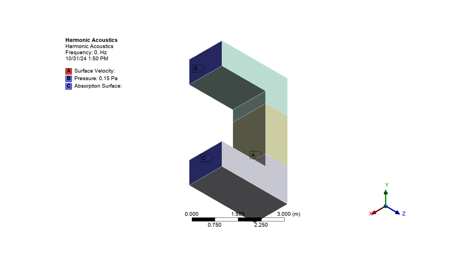
# Activate the harmonic acoustics analysis
harmonic_acoustics.Activate()
# Set the camera to fit the mesh and export the image
set_camera_and_display_image(
camera, graphics, settings_720p, output_path, "bounday_conditions.png", set_fit=True
)
Add results to the harmonic acoustics solution#
# Get the harmonic acoustics solution
solution = model.Analyses[0].Solution
Add the acoustic pressure result
acoustic_pressure_result_1 = solution.AddAcousticPressureResult()
acoustic_pressure_result_1.By = SetDriverStyle.ResultSet
acoustic_pressure_result_1.SetNumber = 25
Add the acoustic total and directional velocity results
# Add the acoustic total velocity result and set its frequency
acoustic_total_velocity_1 = solution.AddAcousticTotalVelocityResult()
acoustic_total_velocity_1.Frequency = Quantity("50 [Hz]")

# Add the acoustic directional velocity result and set its frequency and coordinate system
acoustic_directional_velocity_1 = solution.AddAcousticDirectionalVelocityResult()
acoustic_directional_velocity_1.Frequency = Quantity("50 [Hz]")
acoustic_directional_velocity_1.CoordinateSystem = lcs1

# Add the acoustic total velocity result and set its orientation
acoustic_directional_velocity_2 = solution.AddAcousticDirectionalVelocityResult()
acoustic_directional_velocity_2.NormalOrientation = NormalOrientationType.ZAxis
acoustic_directional_velocity_2.By = SetDriverStyle.ResultSet
acoustic_directional_velocity_2.SetNumber = 25
Add the acoustic sound pressure levels and frequency band responses
# Add the acoustic sound pressure level and set its frequency
acoustic_spl = solution.AddAcousticSoundPressureLevel()
acoustic_spl.Frequency = Quantity("50 [Hz]")

# Add the acoustic A-weighted sound pressure level and set its frequency
acoustic_a_spl = solution.AddAcousticAWeightedSoundPressureLevel()
acoustic_a_spl.Frequency = Quantity("50 [Hz]")

# Add the acoustic frequency band sound pressure level
acoustic_frq_band_spl = solution.AddAcousticFrequencyBandSPL()

# Add the acoustic A-weighted frequency band sound pressure level
a_freq_band_spl = solution.AddAcousticFrequencyBandAWeightedSPL()

# Add the acoustic velocity frequency response and set its orientation and location
z_velocity_response = solution.AddAcousticVelocityFrequencyResponse()
z_velocity_response.NormalOrientation = NormalOrientationType.ZAxis
# Set the location to the pressure face named selection
z_velocity_response.Location = pres_face
Add the acoustic kinetic and potentional energy frequency responses
# Add the acoustic kinetic energy frequency response and set its location
# to the absorption face named selection
ke_response = solution.AddAcousticKineticEnergyFrequencyResponse()
ke_response.Location = abs_face
ke_display = ke_response.TimeHistoryDisplay

# Add the acoustic potential energy frequency response and set its location
# to the absorption face named selection
pe_response = solution.AddAcousticPotentialEnergyFrequencyResponse()
pe_response.Location = abs_face
pe_display = pe_response.TimeHistoryDisplay
Create a function to set the properties of the acoustic velocity result
def set_properties(
    element,
    frequency,
    location,
    amplitude=True,
    normal_orientation=None,
):
    """Set the properties of the acoustic velocity result."""
    element.Frequency = frequency
    element.Amplitude = amplitude
    if normal_orientation:
        element.NormalOrientation = normal_orientation
    # Set the location to the specified named selection
    element.Location = location
    return element
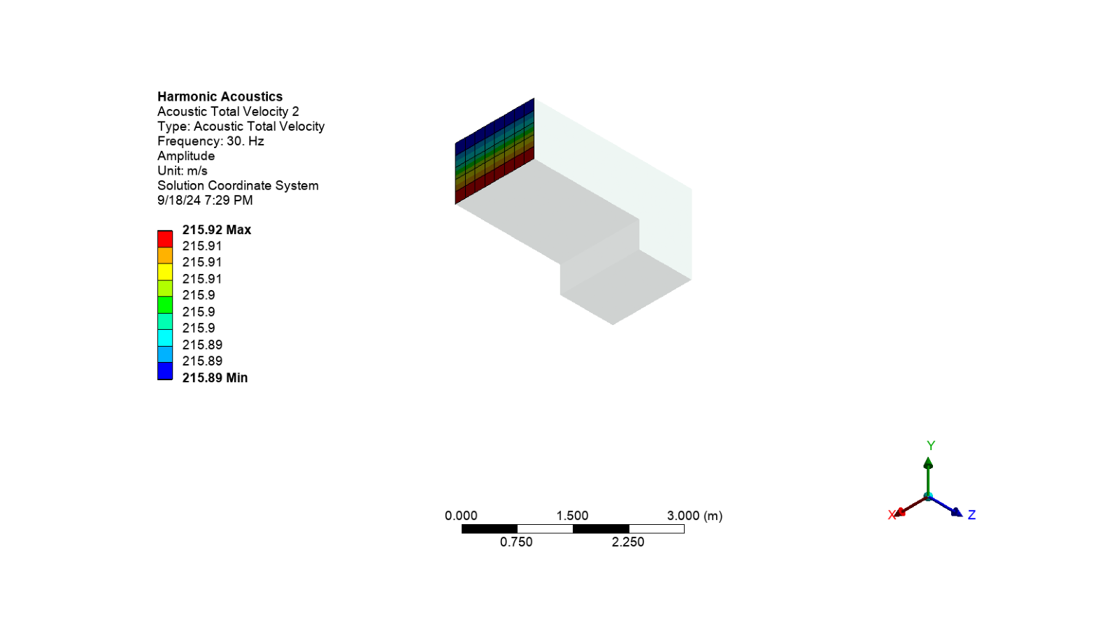
Add the acoustic total and directional velocity results
acoustic_total_velocity_2 = solution.AddAcousticTotalVelocityResult()
set_properties(acoustic_total_velocity_2, Quantity("30 [Hz]"), pres_face)

acoustic_directional_velocity_3 = solution.AddAcousticDirectionalVelocityResult()
set_properties(
    acoustic_directional_velocity_3,
    Quantity("10 [Hz]"),
    pres_face,
    normal_orientation=NormalOrientationType.ZAxis,
)
<Ansys.ACT.Automation.Mechanical.Results.AcousticResults.AcousticDirectionalVelocityResult object at 0x7fdf51d01b00>
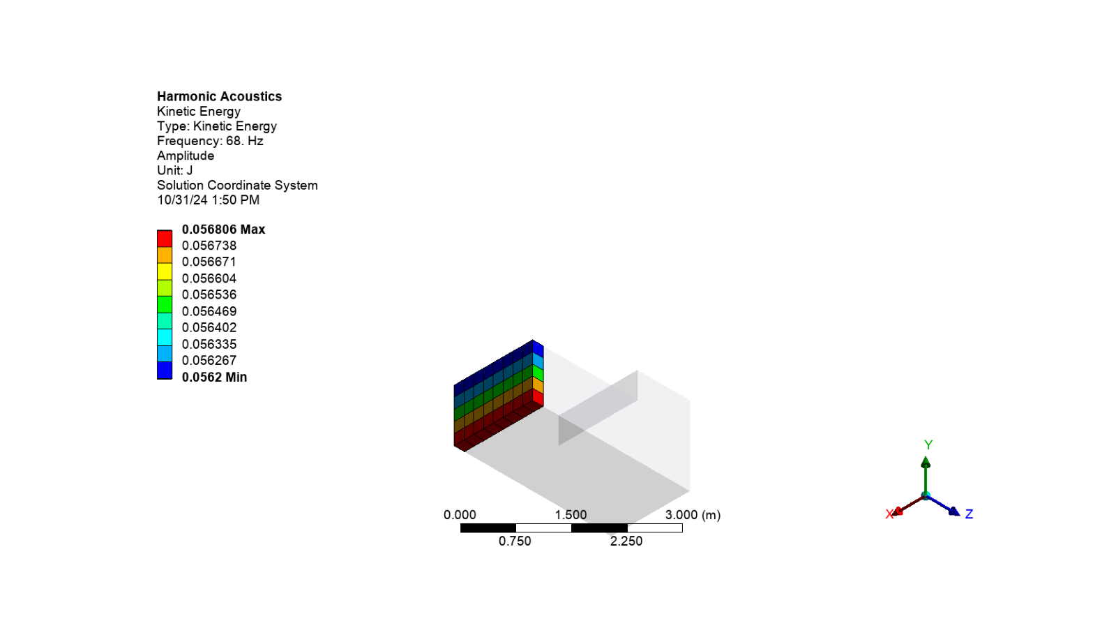
Add the acoustic kinetic and potential energy results
acoustic_ke = solution.AddAcousticKineticEnergy()
set_properties(acoustic_ke, Quantity("68 [Hz]"), abs_face)

acoustic_pe = solution.AddAcousticPotentialEnergy()
set_properties(acoustic_pe, Quantity("10 [Hz]"), abs_face)
<Ansys.ACT.Automation.Mechanical.Results.AcousticResults.AcousticPotentialEnergy object at 0x7fdf51cf0b00>
Solve the harmonic acoustics analysis solution#
solution.Solve(True)
Show messages#
# Print all messages from Mechanical
app.messages.show()
Severity: Warning
DisplayString: Averaged element nodal results when evaluated in the Solution Coordinate System may produce incorrect results (if the nodes/elements involved are aligned differently from each other). Please check your results carefully.
Severity: Warning
DisplayString: Averaged element nodal results when evaluated in the Solution Coordinate System may produce incorrect results (if the nodes/elements involved are aligned differently from each other). Please check your results carefully.
Severity: Warning
DisplayString: One or more Contact Regions are connected to Acoustic Physics Regions. To improve the solution, the contact settings may have been overwritten internally.  Refer to the notes for Acoustics Analysis in the Help System for more details.
Severity: Info
DisplayString: The requested license was received from the License Manager after 22 seconds.
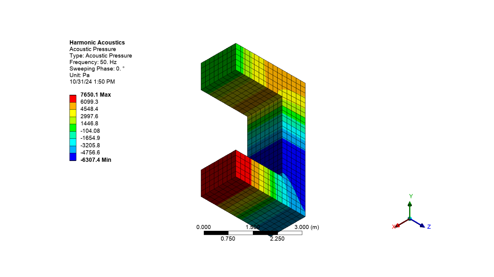
Postprocessing#
Display the total acoustic pressure result
app.Tree.Activate([acoustic_pressure_result_1])
set_camera_and_display_image(
    camera, graphics, settings_720p, output_path, "pressure.png"
)

Display the total acoustic velocity
app.Tree.Activate([acoustic_pressure_result_1])
set_camera_and_display_image(
    camera, graphics, settings_720p, output_path, "total_velocity.png"
)
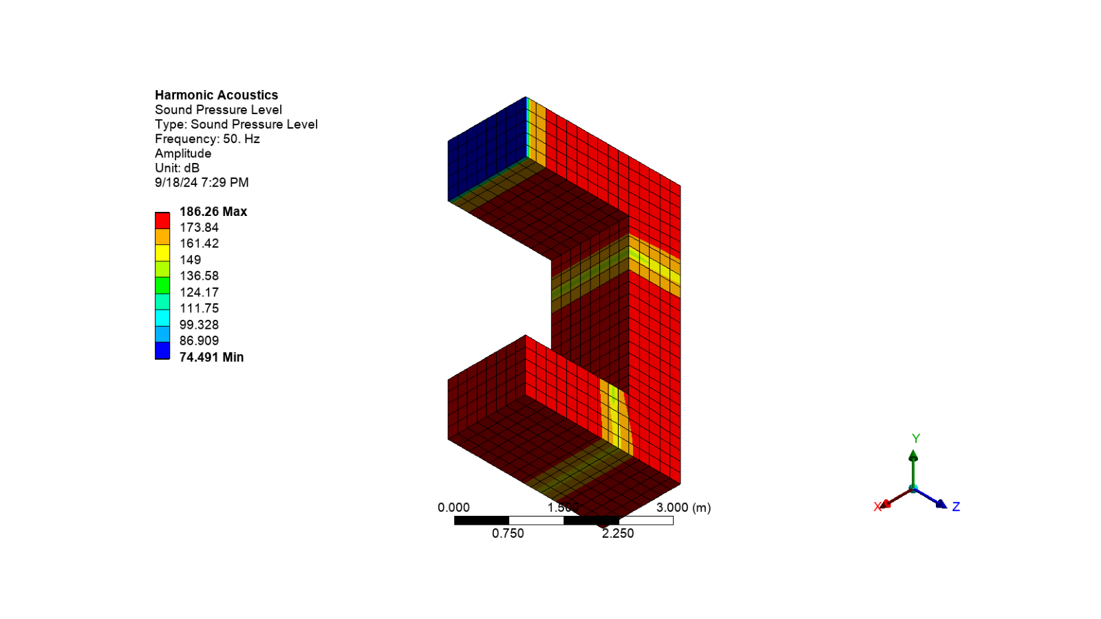
Display the acoustic sound pressure level
app.Tree.Activate([acoustic_spl])
set_camera_and_display_image(
    camera, graphics, settings_720p, output_path, "sound_pressure_level.png"
)
Display the acoustic directional velocity
app.Tree.Activate([acoustic_directional_velocity_3])
set_camera_and_display_image(
    camera, graphics, settings_720p, output_path, "directional_velocity.png"
)
Display the acoustic kinetic energy
app.Tree.Activate([acoustic_ke])
set_camera_and_display_image(
    camera, graphics, settings_720p, output_path, "kinetic_energy.png"
)
Create a function to update the animation frames
def update_animation(frame: int) -> list[mpimg.AxesImage]:
    """Update the animation frame for the GIF.

    Parameters
    ----------
    frame : int
        The frame number to update the animation.

    Returns
    -------
    list[mpimg.AxesImage]
        A list containing the updated image for the animation.
    """
    # Seeks to the given frame in this sequence file
    gif.seek(frame)
    # Set the image array to the current frame of the GIF
    image.set_data(gif.convert("RGBA"))
    # Return the updated image
    return [image]
Display the total acoustic pressure animation
# Set the animation export format to GIF
animation_export_format = (
    Ansys.Mechanical.DataModel.Enums.GraphicsAnimationExportFormat.GIF
)

# Configure the export settings for the animation
settings_720p = Ansys.Mechanical.Graphics.AnimationExportSettings()
settings_720p.Width = 1280
settings_720p.Height = 720

# Export the animation of the acoustic pressure result
press_gif = output_path / "press.gif"
acoustic_pressure_result_1.ExportAnimation(
    str(press_gif), animation_export_format, settings_720p
)

# Open the GIF file and create an animation
gif = Image.open(press_gif)
# Set the subplots for the animation and turn off the axis
figure, axes = plt.subplots(figsize=(16, 9))
axes.axis("off")
# Change the color of the image
image = axes.imshow(gif.convert("RGBA"))

# Create the animation using the figure, update_animation function, and the GIF frames
# Set the interval between frames to 200 milliseconds and repeat the animation
ani = FuncAnimation(
    figure,
    update_animation,
    frames=range(gif.n_frames),
    interval=200,
    repeat=True,
    blit=True,
)

# Show the animation
plt.show()
Display the output file from the solve#
# Get the working directory of the solve
solve_path = harmonic_acoustics.WorkingDir
solve_out_path = Path(solve_path) / "solve.out"

# Check if the solve output file exists and write its contents to the console
if solve_out_path:
    with solve_out_path.open("rt") as file:
        for line in file:
            print(line, end="")
Ansys Mechanical Enterprise
*------------------------------------------------------------------*
| |
| W E L C O M E T O T H E A N S Y S (R) P R O G R A M |
| |
*------------------------------------------------------------------*
***************************************************************
* ANSYS MAPDL 2025 R2 LEGAL NOTICES *
***************************************************************
* *
* Copyright 1971-2025 Ansys, Inc. All rights reserved. *
* Unauthorized use, distribution or duplication is *
* prohibited. *
* *
* Ansys is a registered trademark of Ansys, Inc. or its *
* subsidiaries in the United States or other countries. *
* See the Ansys, Inc. online documentation or the Ansys, Inc. *
* documentation CD or online help for the complete Legal *
* Notice. *
* *
***************************************************************
* *
* THIS ANSYS SOFTWARE PRODUCT AND PROGRAM DOCUMENTATION *
* INCLUDE TRADE SECRETS AND CONFIDENTIAL AND PROPRIETARY *
* PRODUCTS OF ANSYS, INC., ITS SUBSIDIARIES, OR LICENSORS. *
* The software products and documentation are furnished by *
* Ansys, Inc. or its subsidiaries under a software license *
* agreement that contains provisions concerning *
* non-disclosure, copying, length and nature of use, *
* compliance with exporting laws, warranties, disclaimers, *
* limitations of liability, and remedies, and other *
* provisions. The software products and documentation may be *
* used, disclosed, transferred, or copied only in accordance *
* with the terms and conditions of that software license *
* agreement. *
* *
* Ansys, Inc. is a UL registered *
* ISO 9001:2015 company. *
* *
***************************************************************
* *
* This product is subject to U.S. laws governing export and *
* re-export. *
* *
* For U.S. Government users, except as specifically granted *
* by the Ansys, Inc. software license agreement, the use, *
* duplication, or disclosure by the United States Government *
* is subject to restrictions stated in the Ansys, Inc. *
* software license agreement and FAR 12.212 (for non-DOD *
* licenses). *
* *
***************************************************************
2025 R2
Point Releases and Patches installed:
Ansys, Inc. License Manager 2025 R2
LS-DYNA 2025 R2
Core WB Files 2025 R2
Mechanical Products 2025 R2
***** MAPDL COMMAND LINE ARGUMENTS *****
BATCH MODE REQUESTED (-b) = NOLIST
INPUT FILE COPY MODE (-c) = COPY
DISTRIBUTED MEMORY PARALLEL REQUESTED
4 PARALLEL PROCESSES REQUESTED WITH SINGLE THREAD PER PROCESS
TOTAL OF 4 CORES REQUESTED
INPUT FILE NAME = /github/home/.mw/Application Data/Ansys/v252/AnsysMechCC4F/Project_Mech_Files/HarmonicAcoustics/dummy.dat
OUTPUT FILE NAME = /github/home/.mw/Application Data/Ansys/v252/AnsysMechCC4F/Project_Mech_Files/HarmonicAcoustics/solve.out
START-UP FILE MODE = NOREAD
STOP FILE MODE = NOREAD
RELEASE= 2025 R2 BUILD= 25.2 UP20250519 VERSION=LINUX x64
CURRENT JOBNAME=file0 09:08:40 JUL 17, 2025 CP= 0.232
PARAMETER _DS_PROGRESS = 999.0000000
/INPUT FILE= ds.dat LINE= 0
*** NOTE *** CP = 0.338 TIME= 09:08:40
The /CONFIG,NOELDB command is not valid in a distributed memory
parallel solution. Command is ignored.
*GET _WALLSTRT FROM ACTI ITEM=TIME WALL VALUE= 9.14444444
TITLE=
--Harmonic Acoustics
SET PARAMETER DIMENSIONS ON _WB_PROJECTSCRATCH_DIR
TYPE=STRI DIMENSIONS= 248 1 1
PARAMETER _WB_PROJECTSCRATCH_DIR(1) = /github/home/.mw/Application Data/Ansys/v252/AnsysMechCC4F/Project_Mech_Files/HarmonicAcoustics/
SET PARAMETER DIMENSIONS ON _WB_SOLVERFILES_DIR
TYPE=STRI DIMENSIONS= 248 1 1
PARAMETER _WB_SOLVERFILES_DIR(1) = /github/home/.mw/Application Data/Ansys/v252/AnsysMechCC4F/Project_Mech_Files/HarmonicAcoustics/
SET PARAMETER DIMENSIONS ON _WB_USERFILES_DIR
TYPE=STRI DIMENSIONS= 248 1 1
PARAMETER _WB_USERFILES_DIR(1) = /github/home/.mw/Application Data/Ansys/v252/AnsysMechCC4F/Project_Mech_Files/UserFiles/
--- Data in consistent MKS units. See Solving Units in the help system for more
MKS UNITS SPECIFIED FOR INTERNAL
LENGTH (l) = METER (M)
MASS (M) = KILOGRAM (KG)
TIME (t) = SECOND (SEC)
TEMPERATURE (T) = CELSIUS (C)
TOFFSET = 273.0
CHARGE (Q) = COULOMB
FORCE (f) = NEWTON (N) (KG-M/SEC2)
HEAT = JOULE (N-M)
PRESSURE = PASCAL (NEWTON/M**2)
ENERGY (W) = JOULE (N-M)
POWER (P) = WATT (N-M/SEC)
CURRENT (i) = AMPERE (COULOMBS/SEC)
CAPACITANCE (C) = FARAD
INDUCTANCE (L) = HENRY
MAGNETIC FLUX = WEBER
RESISTANCE (R) = OHM
ELECTRIC POTENTIAL = VOLT
INPUT UNITS ARE ALSO SET TO MKS
*** MAPDL - ENGINEERING ANALYSIS SYSTEM RELEASE 2025 R2 25.2 ***
Ansys Mechanical Enterprise
00000000 VERSION=LINUX x64 09:08:40 JUL 17, 2025 CP= 0.342
--Harmonic Acoustics
***** MAPDL ANALYSIS DEFINITION (PREP7) *****
*********** Send User Defined Coordinate System(s) ***********
*********** Nodes for the whole assembly ***********
*********** Elements for Body 1 'Solid' ***********
*********** Elements for Body 2 'Solid' ***********
*********** Elements for Body 3 'Solid' ***********
*********** Set Reference Temperature ***********
*********** Send Materials ***********
*********** Create Contact "Contact Region 6" ***********
Real Constant Set For Above Contact Is 5 & 4
*********** Create Contact "Contact Region 9" ***********
Real Constant Set For Above Contact Is 7 & 6
*********** Send Named Selection as Node Component ***********
*********** Send Named Selection as Node Component ***********
*********** Send Named Selection as Node Component ***********
*********** Send Named Selection as Element Component ***********
*********** Create Acoustic Pressure ***********
*********** Create Absorption Surface ***********
*********** Begin Program Controlled Acoustic Far-field Radiation Surface *****
*********** End Program Controlled Acoustic Far-field Radiation Surface *******
*********** Create Surface Velocity ***********
***** ROUTINE COMPLETED ***** CP = 0.494
--- Number of total nodes = 9687
--- Number of contact elements = 320
--- Number of spring elements = 0
--- Number of bearing elements = 0
--- Number of solid elements = 1840
--- Number of condensed parts = 0
--- Number of total elements = 2160
*GET _WALLBSOL FROM ACTI ITEM=TIME WALL VALUE= 9.14444444
***** MAPDL SOLUTION ROUTINE *****
PERFORM A HARMONIC ANALYSIS
THIS WILL BE A NEW ANALYSIS
PERFORM A FULL HARMONIC RESPONSE ANALYSIS
THERMAL STRAINS ARE NOT INCLUDED IN THE LOAD VECTOR.
STEP BOUNDARY CONDITION KEY= 1
HARMONIC FREQUENCY RANGE - END= 100.00 BEGIN= 0.0000
USE 50 SUBSTEP(S) THIS LOAD STEP FOR ALL DEGREES OF FREEDOM
*** NOTE *** CP = 0.499 TIME= 09:08:40
The acoustic solver is set to the total field formulation.
ERASE THE CURRENT DATABASE OUTPUT CONTROL TABLE.
WRITE ALL ITEMS TO THE DATABASE WITH A FREQUENCY OF NONE
FOR ALL APPLICABLE ENTITIES
WRITE NSOL ITEMS TO THE DATABASE WITH A FREQUENCY OF ALL
FOR ALL APPLICABLE ENTITIES
WRITE EANG ITEMS TO THE DATABASE WITH A FREQUENCY OF ALL
FOR ALL APPLICABLE ENTITIES
WRITE ETMP ITEMS TO THE DATABASE WITH A FREQUENCY OF ALL
FOR ALL APPLICABLE ENTITIES
WRITE VENG ITEMS TO THE DATABASE WITH A FREQUENCY OF ALL
FOR ALL APPLICABLE ENTITIES
PRINTOUT RESUMED BY /GOP
WRITE MISC ITEMS TO THE DATABASE WITH A FREQUENCY OF ALL
FOR THE ENTITIES DEFINED BY COMPONENT _ELMISC
WRITE FGRA ITEMS TO THE DATABASE WITH A FREQUENCY OF ALL
FOR ALL APPLICABLE ENTITIES
*GET ANSINTER_ FROM ACTI ITEM=INT VALUE= 0.00000000
*IF ANSINTER_ ( = 0.00000 ) NE
0 ( = 0.00000 ) THEN
*ENDIF
*** NOTE *** CP = 0.542 TIME= 09:08:40
The automatic domain decomposition logic has selected the FREQ domain
decomposition method with 1 processes per frequency solution.
***** MAPDL SOLVE COMMAND *****
D I S T R I B U T E D D O M A I N D E C O M P O S E R
...Number of frequency solutions: 50
...Decompose to 4 frequency domains (with 1 processes per domain)
*** WARNING *** CP = 0.728 TIME= 09:08:40
Element shape checking is currently inactive. Issue SHPP,ON or
SHPP,WARN to reactivate, if desired.
*** NOTE *** CP = 0.742 TIME= 09:08:40
The model data was checked and warning messages were found.
Please review output or errors file ( /github/home/.mw/Application
Data/Ansys/v252/AnsysMechCC4F/Project_Mech_Files/HarmonicAcoustics/file
e0.err ) for these warning messages.
*** MAPDL - ENGINEERING ANALYSIS SYSTEM RELEASE 2025 R2 25.2 ***
Ansys Mechanical Enterprise
00000000 VERSION=LINUX x64 09:08:40 JUL 17, 2025 CP= 0.743
--Harmonic Acoustics
S O L U T I O N O P T I O N S
PROBLEM DIMENSIONALITY. . . . . . . . . . . . .3-D
DEGREES OF FREEDOM. . . . . . PRES
ANALYSIS TYPE . . . . . . . . . . . . . . . . .HARMONIC
SOLUTION METHOD. . . . . . . . . . . . . . .AUTO
OFFSET TEMPERATURE FROM ABSOLUTE ZERO . . . . . 273.15
THERMAL EXPANSION . . . . . . . . . . . . . . .OFF
COMPLEX DISPLACEMENT PRINT OPTION . . . . . . .REAL AND IMAGINARY
GLOBALLY ASSEMBLED MATRIX . . . . . . . . . . .SYMMETRIC
*** NOTE *** CP = 0.757 TIME= 09:08:40
The Solution Control Option is only valid for single field structural,
single field thermal, single field diffusion, coupled
thermal-diffusion analyses and coupled-field analyses with structural
degrees of freedom. The SOLCONTROL,ON command (if present) has been
de-activated.
*** NOTE *** CP = 0.787 TIME= 09:08:40
A target element 3397 is attached to a fluid element 1836. You may
consider to flip the contact and target surfaces.
*** NOTE *** CP = 1.579 TIME= 09:08:41
Symmetric Deformable- deformable contact pair identified by real
constant set 4 and contact element type 4 has been set up. The
companion pair has real constant set ID 5. Both pairs should have the
same behavior.
*WARNING*: The contact pairs have similar mesh patterns. MAPDL will
keep the current pair and deactivate its companion pair.
Pure pore fluid contact is activated.
Contact algorithm: MPC based approach
*** NOTE *** CP = 1.579 TIME= 09:08:41
Contact related postprocess items (ETABLE, pressure ...) are not
available.
Contact detection at: nodal point (surface projection based)
MPC will be built internally to handle bonded contact.
Average contact surface length 0.19070
Average contact pair depth 0.17708
Average target surface length 0.19375
Default pinball region factor PINB 0.25000
The resulting pinball region 0.44271E-01
Initial penetration/gap is excluded.
Bonded contact (always) is defined.
*** NOTE *** CP = 1.579 TIME= 09:08:41
Max. Initial penetration 2.852608047E-15 was detected between contact
element 3333 and target element 3413.
****************************************
*** WARNING *** CP = 1.580 TIME= 09:08:41
Element shape checking is currently inactive. Issue SHPP,ON or
SHPP,WARN to reactivate, if desired.
*** WARNING *** CP = 1.580 TIME= 09:08:41
Element shape checking is currently inactive. Issue SHPP,ON or
SHPP,WARN to reactivate, if desired.
*** WARNING *** CP = 1.580 TIME= 09:08:41
Element shape checking is currently inactive. Issue SHPP,ON or
SHPP,WARN to reactivate, if desired.
*** NOTE *** CP = 1.580 TIME= 09:08:41
Symmetric Deformable- deformable contact pair identified by real
constant set 5 and contact element type 4 has been set up. The
companion pair has real constant set ID 4. Both pairs should have the
same behavior.
MAPDL will deactivate the current pair and keep its companion pair,
resulting in asymmetric contact.
Pure pore fluid contact is activated.
Contact algorithm: MPC based approach
*** NOTE *** CP = 1.580 TIME= 09:08:41
Contact related postprocess items (ETABLE, pressure ...) are not
available.
Contact detection at: nodal point (surface projection based)
MPC will be built internally to handle bonded contact.
Average contact surface length 0.19070
Average contact pair depth 0.20000
Average target surface length 0.19375
Default pinball region factor PINB 0.25000
The resulting pinball region 0.50000E-01
Initial penetration/gap is excluded.
Bonded contact (always) is defined.
*** NOTE *** CP = 1.580 TIME= 09:08:41
Max. Initial penetration 2.404977522E-15 was detected between contact
element 3381 and target element 3285.
****************************************
*** NOTE *** CP = 1.580 TIME= 09:08:41
Symmetric Deformable- deformable contact pair identified by real
constant set 6 and contact element type 6 has been set up. The
companion pair has real constant set ID 7. Both pairs should have the
same behavior.
*WARNING*: The contact pairs have similar mesh patterns. MAPDL will
keep the current pair and deactivate its companion pair.
Pure pore fluid contact is activated.
Contact algorithm: MPC based approach
*** NOTE *** CP = 1.580 TIME= 09:08:41
Contact related postprocess items (ETABLE, pressure ...) are not
available.
Contact detection at: nodal point (surface projection based)
MPC will be built internally to handle bonded contact.
Average contact surface length 0.19070
Average contact pair depth 0.17708
Average target surface length 0.19375
Default pinball region factor PINB 0.25000
The resulting pinball region 0.44271E-01
Initial penetration/gap is excluded.
Bonded contact (always) is defined.
*** NOTE *** CP = 1.580 TIME= 09:08:41
Max. Initial penetration 1.025113101E-15 was detected between contact
element 3502 and target element 3587.
****************************************
*** NOTE *** CP = 1.580 TIME= 09:08:41
Symmetric Deformable- deformable contact pair identified by real
constant set 7 and contact element type 6 has been set up. The
companion pair has real constant set ID 6. Both pairs should have the
same behavior.
MAPDL will deactivate the current pair and keep its companion pair,
resulting in asymmetric contact.
Pure pore fluid contact is activated.
Contact algorithm: MPC based approach
*** NOTE *** CP = 1.580 TIME= 09:08:41
Contact related postprocess items (ETABLE, pressure ...) are not
available.
Contact detection at: nodal point (surface projection based)
MPC will be built internally to handle bonded contact.
Average contact surface length 0.19070
Average contact pair depth 0.20000
Average target surface length 0.19375
Default pinball region factor PINB 0.25000
The resulting pinball region 0.50000E-01
Initial penetration/gap is excluded.
Bonded contact (always) is defined.
*** NOTE *** CP = 1.580 TIME= 09:08:41
Max. Initial penetration 1.419491659E-15 was detected between contact
element 3525 and target element 3452.
****************************************
L O A D S T E P O P T I O N S
LOAD STEP NUMBER. . . . . . . . . . . . . . . . 1
FREQUENCY RANGE . . . . . . . . . . . . . . . . 0.0000 TO 100.00
NUMBER OF SUBSTEPS. . . . . . . . . . . . . . . 50
STEP CHANGE BOUNDARY CONDITIONS . . . . . . . . YES
PRINT OUTPUT CONTROLS . . . . . . . . . . . . .NO PRINTOUT
DATABASE OUTPUT CONTROLS
ITEM FREQUENCY COMPONENT
ALL NONE
NSOL ALL
EANG ALL
ETMP ALL
VENG ALL
MISC ALL _ELMISC
FGRA ALL
AUTO SELECTION OF VT FOR FREQUENCY SWEEP. . . . NO
*** NOTE *** CP = 2.451 TIME= 09:08:41
Symmetric Deformable- deformable contact pair identified by real
constant set 4 and contact element type 4 has been set up. The
companion pair has real constant set ID 5. Both pairs should have the
same behavior.
MAPDL will keep the current pair and deactivate its companion pair,
resulting in asymmetric contact.
Pure pore fluid contact is activated.
Contact algorithm: MPC based approach
*** NOTE *** CP = 2.451 TIME= 09:08:41
Contact related postprocess items (ETABLE, pressure ...) are not
available.
Contact detection at: nodal point (surface projection based)
MPC will be built internally to handle bonded contact.
Average contact surface length 0.19070
Average contact pair depth 0.17708
Average target surface length 0.19375
Default pinball region factor PINB 0.25000
The resulting pinball region 0.44271E-01
Initial penetration/gap is excluded.
Bonded contact (always) is defined.
*** NOTE *** CP = 2.451 TIME= 09:08:41
Max. Initial penetration 2.852608047E-15 was detected between contact
element 3333 and target element 3413.
****************************************
*** NOTE *** CP = 2.452 TIME= 09:08:41
Symmetric Deformable- deformable contact pair identified by real
constant set 5 and contact element type 4 has been set up. The
companion pair has real constant set ID 4. Both pairs should have the
same behavior.
MAPDL will deactivate the current pair and keep its companion pair,
resulting in asymmetric contact.
Pure pore fluid contact is activated.
Contact algorithm: MPC based approach
*** NOTE *** CP = 2.452 TIME= 09:08:41
Contact related postprocess items (ETABLE, pressure ...) are not
available.
Contact detection at: nodal point (surface projection based)
MPC will be built internally to handle bonded contact.
Average contact surface length 0.19070
Average contact pair depth 0.20000
Average target surface length 0.19375
Default pinball region factor PINB 0.25000
The resulting pinball region 0.50000E-01
Initial penetration/gap is excluded.
Bonded contact (always) is defined.
*** NOTE *** CP = 2.452 TIME= 09:08:41
Max. Initial penetration 2.404977522E-15 was detected between contact
element 3381 and target element 3285.
****************************************
*** NOTE *** CP = 2.452 TIME= 09:08:41
Symmetric Deformable- deformable contact pair identified by real
constant set 6 and contact element type 6 has been set up. The
companion pair has real constant set ID 7. Both pairs should have the
same behavior.
MAPDL will keep the current pair and deactivate its companion pair,
resulting in asymmetric contact.
Pure pore fluid contact is activated.
Contact algorithm: MPC based approach
*** NOTE *** CP = 2.452 TIME= 09:08:41
Contact related postprocess items (ETABLE, pressure ...) are not
available.
Contact detection at: nodal point (surface projection based)
MPC will be built internally to handle bonded contact.
Average contact surface length 0.19070
Average contact pair depth 0.17708
Average target surface length 0.19375
Default pinball region factor PINB 0.25000
The resulting pinball region 0.44271E-01
Initial penetration/gap is excluded.
Bonded contact (always) is defined.
*** NOTE *** CP = 2.452 TIME= 09:08:41
Max. Initial penetration 1.025113101E-15 was detected between contact
element 3502 and target element 3587.
****************************************
*** NOTE *** CP = 2.452 TIME= 09:08:41
Symmetric Deformable- deformable contact pair identified by real
constant set 7 and contact element type 6 has been set up. The
companion pair has real constant set ID 6. Both pairs should have the
same behavior.
MAPDL will deactivate the current pair and keep its companion pair,
resulting in asymmetric contact.
Pure pore fluid contact is activated.
Contact algorithm: MPC based approach
*** NOTE *** CP = 2.452 TIME= 09:08:41
Contact related postprocess items (ETABLE, pressure ...) are not
available.
Contact detection at: nodal point (surface projection based)
MPC will be built internally to handle bonded contact.
Average contact surface length 0.19070
Average contact pair depth 0.20000
Average target surface length 0.19375
Default pinball region factor PINB 0.25000
The resulting pinball region 0.50000E-01
Initial penetration/gap is excluded.
Bonded contact (always) is defined.
*** NOTE *** CP = 2.452 TIME= 09:08:41
Max. Initial penetration 1.419491659E-15 was detected between contact
element 3525 and target element 3452.
****************************************
**** CENTER OF MASS, MASS, AND MASS MOMENTS OF INERTIA ****
CALCULATIONS ASSUME ELEMENT MASS AT ELEMENT CENTROID
TOTAL MASS = 16.537
MOM. OF INERTIA MOM. OF INERTIA
CENTER OF MASS ABOUT ORIGIN ABOUT CENTER OF MASS
XC = 0.75000 IXX = 3329. IXX = 61.45
YC = 2.5000 IYY = 3189. IYY = 15.40
ZC = 13.833 IZZ = 164.8 IZZ = 52.15
IXY = -31.01 IXY = 0.2558E-12
IYZ = -571.9 IYZ = 0.6594E-11
IZX = -171.6 IZX = 0.2018E-11
*** MASS SUMMARY BY ELEMENT TYPE ***
TYPE MASS
1 6.43125
2 6.43125
3 3.67500
Range of element maximum matrix coefficients in global coordinates
Maximum = 0.195402284 at element 1153.
Minimum = 0.18606905 at element 1433.
*** ELEMENT MATRIX FORMULATION TIMES
TYPE NUMBER ENAME TOTAL CP AVE CP
1 720 FLUID220 0.062 0.000086
2 720 FLUID220 0.060 0.000083
3 400 FLUID220 0.034 0.000086
4 80 CONTA174 0.011 0.000140
5 80 TARGE170 0.000 0.000005
6 80 CONTA174 0.011 0.000132
7 80 TARGE170 0.000 0.000005
Time at end of element matrix formulation CP = 2.75799084.
SPARSE MATRIX DIRECT SOLVER.
Number of equations = 9246, Maximum wavefront = 81
Memory allocated on this process
-------------------------------------------------------------------
Equation solver memory allocated = 52.773 MB
Equation solver memory required for in-core mode = 50.566 MB
Equation solver memory required for out-of-core mode = 21.577 MB
Total (solver and non-solver) memory allocated = 636.000 MB
*** NOTE *** CP = 2.893 TIME= 09:08:41
The Sparse Matrix Solver is currently running in the in-core memory
mode. This memory mode uses the most amount of memory in order to
avoid using the hard drive as much as possible, which most often
results in the fastest solution time. This mode is recommended if
enough physical memory is present to accommodate all of the solver
data.
Sparse solver maximum pivot= 0.772343337 at node 1569 PRES.
Sparse solver minimum pivot= 0.104583107 at node 646 PRES.
Sparse solver minimum pivot in absolute value= 0.104583107 at node 646
PRES.
*** ELEMENT RESULT CALCULATION TIMES
TYPE NUMBER ENAME TOTAL CP AVE CP
1 720 FLUID220 0.056 0.000077
2 720 FLUID220 0.058 0.000080
3 400 FLUID220 0.031 0.000078
*** NODAL LOAD CALCULATION TIMES
TYPE NUMBER ENAME TOTAL CP AVE CP
1 720 FLUID220 0.004 0.000006
2 720 FLUID220 0.004 0.000006
3 400 FLUID220 0.002 0.000006
*** LOAD STEP 1 SUBSTEP 1 COMPLETED. FREQUENCY= 2.00000
*** LOAD STEP 1 SUBSTEP 2 COMPLETED. FREQUENCY= 4.00000
*** LOAD STEP 1 SUBSTEP 3 COMPLETED. FREQUENCY= 6.00000
*** LOAD STEP 1 SUBSTEP 4 COMPLETED. FREQUENCY= 8.00000
*** LOAD STEP 1 SUBSTEP 5 COMPLETED. FREQUENCY= 10.0000
*** LOAD STEP 1 SUBSTEP 6 COMPLETED. FREQUENCY= 12.0000
*** LOAD STEP 1 SUBSTEP 7 COMPLETED. FREQUENCY= 14.0000
*** LOAD STEP 1 SUBSTEP 8 COMPLETED. FREQUENCY= 16.0000
*** LOAD STEP 1 SUBSTEP 9 COMPLETED. FREQUENCY= 18.0000
*** LOAD STEP 1 SUBSTEP 10 COMPLETED. FREQUENCY= 20.0000
*** LOAD STEP 1 SUBSTEP 11 COMPLETED. FREQUENCY= 22.0000
*** LOAD STEP 1 SUBSTEP 12 COMPLETED. FREQUENCY= 24.0000
*** LOAD STEP 1 SUBSTEP 13 COMPLETED. FREQUENCY= 26.0000
*** LOAD STEP 1 SUBSTEP 14 COMPLETED. FREQUENCY= 28.0000
*** LOAD STEP 1 SUBSTEP 15 COMPLETED. FREQUENCY= 30.0000
*** LOAD STEP 1 SUBSTEP 16 COMPLETED. FREQUENCY= 32.0000
*** LOAD STEP 1 SUBSTEP 17 COMPLETED. FREQUENCY= 34.0000
*** LOAD STEP 1 SUBSTEP 18 COMPLETED. FREQUENCY= 36.0000
*** LOAD STEP 1 SUBSTEP 19 COMPLETED. FREQUENCY= 38.0000
*** LOAD STEP 1 SUBSTEP 20 COMPLETED. FREQUENCY= 40.0000
*** LOAD STEP 1 SUBSTEP 21 COMPLETED. FREQUENCY= 42.0000
*** LOAD STEP 1 SUBSTEP 22 COMPLETED. FREQUENCY= 44.0000
*** LOAD STEP 1 SUBSTEP 23 COMPLETED. FREQUENCY= 46.0000
*** LOAD STEP 1 SUBSTEP 24 COMPLETED. FREQUENCY= 48.0000
*** LOAD STEP 1 SUBSTEP 25 COMPLETED. FREQUENCY= 50.0000
*** LOAD STEP 1 SUBSTEP 26 COMPLETED. FREQUENCY= 52.0000
*** LOAD STEP 1 SUBSTEP 27 COMPLETED. FREQUENCY= 54.0000
*** LOAD STEP 1 SUBSTEP 28 COMPLETED. FREQUENCY= 56.0000
*** LOAD STEP 1 SUBSTEP 29 COMPLETED. FREQUENCY= 58.0000
*** LOAD STEP 1 SUBSTEP 30 COMPLETED. FREQUENCY= 60.0000
*** LOAD STEP 1 SUBSTEP 31 COMPLETED. FREQUENCY= 62.0000
*** LOAD STEP 1 SUBSTEP 32 COMPLETED. FREQUENCY= 64.0000
*** LOAD STEP 1 SUBSTEP 33 COMPLETED. FREQUENCY= 66.0000
*** LOAD STEP 1 SUBSTEP 34 COMPLETED. FREQUENCY= 68.0000
*** LOAD STEP 1 SUBSTEP 35 COMPLETED. FREQUENCY= 70.0000
*** LOAD STEP 1 SUBSTEP 36 COMPLETED. FREQUENCY= 72.0000
*** LOAD STEP 1 SUBSTEP 37 COMPLETED. FREQUENCY= 74.0000
*** LOAD STEP 1 SUBSTEP 38 COMPLETED. FREQUENCY= 76.0000
*** LOAD STEP 1 SUBSTEP 39 COMPLETED. FREQUENCY= 78.0000
*** LOAD STEP 1 SUBSTEP 40 COMPLETED. FREQUENCY= 80.0000
*** LOAD STEP 1 SUBSTEP 41 COMPLETED. FREQUENCY= 82.0000
*** LOAD STEP 1 SUBSTEP 42 COMPLETED. FREQUENCY= 84.0000
*** LOAD STEP 1 SUBSTEP 43 COMPLETED. FREQUENCY= 86.0000
*** LOAD STEP 1 SUBSTEP 44 COMPLETED. FREQUENCY= 88.0000
*** LOAD STEP 1 SUBSTEP 45 COMPLETED. FREQUENCY= 90.0000
*** LOAD STEP 1 SUBSTEP 46 COMPLETED. FREQUENCY= 92.0000
*** LOAD STEP 1 SUBSTEP 47 COMPLETED. FREQUENCY= 94.0000
*** LOAD STEP 1 SUBSTEP 48 COMPLETED. FREQUENCY= 96.0000
*** LOAD STEP 1 SUBSTEP 49 COMPLETED. FREQUENCY= 98.0000
*** LOAD STEP 1 SUBSTEP 50 COMPLETED. FREQUENCY= 100.000
*** MAPDL BINARY FILE STATISTICS
BUFFER SIZE USED= 16384
9.875 MB WRITTEN ON ELEMENT MATRIX FILE: file0.emat
4.125 MB WRITTEN ON ELEMENT SAVED DATA FILE: file0.esav
6.188 MB WRITTEN ON ASSEMBLED MATRIX FILE: file0.full
20.625 MB WRITTEN ON RESULTS FILE: file0.rst
*************** Write FE CONNECTORS *********
WRITE OUT CONSTRAINT EQUATIONS TO FILE= file.ce
FINISH SOLUTION PROCESSING
***** ROUTINE COMPLETED ***** CP = 10.145
PRINTOUT RESUMED BY /GOP
*GET _WALLASOL FROM ACTI ITEM=TIME WALL VALUE= 9.14694444
*** MAPDL - ENGINEERING ANALYSIS SYSTEM RELEASE 2025 R2 25.2 ***
Ansys Mechanical Enterprise
00000000 VERSION=LINUX x64 09:08:49 JUL 17, 2025 CP= 10.147
--Harmonic Acoustics
***** MAPDL RESULTS INTERPRETATION (POST1) *****
*** NOTE *** CP = 10.148 TIME= 09:08:49
Reading results into the database (SET command) will update the current
displacement and force boundary conditions in the database with the
values from the results file for that load set. Note that any
subsequent solutions will use these values unless action is taken to
either SAVE the current values or not overwrite them (/EXIT,NOSAVE).
Set Encoding of XML File to:ISO-8859-1
Set Output of XML File to:
PARM, , , , , , , , , , , ,
, , , , , , ,
DATABASE WRITTEN ON FILE parm.xml
EXIT THE MAPDL POST1 DATABASE PROCESSOR
***** ROUTINE COMPLETED ***** CP = 10.148
PRINTOUT RESUMED BY /GOP
*GET _WALLDONE FROM ACTI ITEM=TIME WALL VALUE= 9.14694444
PARAMETER _PREPTIME = 0.000000000
PARAMETER _SOLVTIME = 9.000000000
PARAMETER _POSTTIME = 0.000000000
PARAMETER _TOTALTIM = 9.000000000
*GET _DLBRATIO FROM ACTI ITEM=SOLU DLBR VALUE= 0.00000000
*GET _COMBTIME FROM ACTI ITEM=SOLU COMB VALUE= 0.766539918E-01
*GET _SSMODE FROM ACTI ITEM=SOLU SSMM VALUE= 2.00000000
*GET _NDOFS FROM ACTI ITEM=SOLU NDOF VALUE= 9246.00000
/FCLEAN COMMAND REMOVING ALL LOCAL FILES
--- Total number of nodes = 9687
--- Total number of elements = 2160
--- Element load balance ratio = 0
--- Time to combine distributed files = 7.665399183E-02
--- Sparse memory mode = 2
--- Number of DOF = 9246
EXIT MAPDL WITHOUT SAVING DATABASE
NUMBER OF WARNING MESSAGES ENCOUNTERED= 4
NUMBER OF ERROR MESSAGES ENCOUNTERED= 0
+--------------------- M A P D L S T A T I S T I C S ------------------------+
Release: 2025 R2 Build: 25.2 Update: UP20250519 Platform: LINUX x64
Date Run: 07/17/2025 Time: 09:08 Process ID: 11423
Operating System: Ubuntu 20.04.6 LTS
Processor Model: AMD EPYC 7763 64-Core Processor
Compiler: Intel(R) Fortran Compiler Classic Version 2021.9 (Build: 20230302)
Intel(R) C/C++ Compiler Classic Version 2021.9 (Build: 20230302)
AOCL-BLAS 5.0.1 Build 20250320
Number of machines requested : 1
Total number of cores available : 8
Number of physical cores available : 4
Number of processes requested : 4
Number of threads per process requested : 1
Total number of cores requested : 4 (Distributed Memory Parallel)
MPI Type: OPENMPI
MPI Version: Open MPI v4.0.5
GPU Acceleration: Not Requested
Job Name: file0
Input File: dummy.dat
Core Machine Name Working Directory
-----------------------------------------------------
0 426ea999332e /github/home/.mw/Application Data/Ansys/v252/AnsysMechCC4F/Project_Mech_Files/HarmonicAcoustics
1 426ea999332e /github/home/.mw/Application Data/Ansys/v252/AnsysMechCC4F/Project_Mech_Files/HarmonicAcoustics
2 426ea999332e /github/home/.mw/Application Data/Ansys/v252/AnsysMechCC4F/Project_Mech_Files/HarmonicAcoustics
3 426ea999332e /github/home/.mw/Application Data/Ansys/v252/AnsysMechCC4F/Project_Mech_Files/HarmonicAcoustics
Latency time from master to core 1 = 2.358 microseconds
Latency time from master to core 2 = 2.084 microseconds
Latency time from master to core 3 = 2.378 microseconds
Communication speed from master to core 1 = 16957.93 MB/sec
Communication speed from master to core 2 = 18353.52 MB/sec
Communication speed from master to core 3 = 20200.65 MB/sec
Total CPU time for main thread : 8.6 seconds
Total CPU time summed for all threads : 10.2 seconds
Elapsed time spent obtaining a license : 0.4 seconds
Elapsed time spent pre-processing model (/PREP7) : 0.0 seconds
Elapsed time spent solution - preprocessing : 0.3 seconds
Elapsed time spent computing solution : 7.8 seconds
Elapsed time spent solution - postprocessing : 0.1 seconds
Elapsed time spent post-processing model (/POST1) : 0.0 seconds
Equation solver used : Sparse (symmetric)
Equation solver computational rate : 5.2 Gflops
Sum of disk space used on all processes : 217.9 MB
Sum of memory used on all processes : 333.0 MB
Sum of memory allocated on all processes : 2880.0 MB
Physical memory available : 31 GB
Total amount of I/O written to disk : 0.9 GB
Total amount of I/O read from disk : 1.8 GB
+------------------ E N D M A P D L S T A T I S T I C S -------------------+
*-----------------------------------------------------------------------------*
| |
| RUN COMPLETED |
| |
|-----------------------------------------------------------------------------|
| |
| Ansys MAPDL 2025 R2 Build 25.2 UP20250519 LINUX x64 |
| |
|-----------------------------------------------------------------------------|
| |
| Database Requested(-db) 1024 MB Scratch Memory Requested 1024 MB |
| Max Database Used(Master) 5 MB Max Scratch Used(Master) 79 MB |
| Max Database Used(Workers) 5 MB Max Scratch Used(Workers) 78 MB |
| Sum Database Used(All) 20 MB Sum Scratch Used(All) 313 MB |
| |
|-----------------------------------------------------------------------------|
| |
| CP Time (sec) = 10.186 Time = 09:08:49 |
| Elapsed Time (sec) = 10.000 Date = 07/17/2025 |
| |
*-----------------------------------------------------------------------------*
Print the project tree#
app.print_tree()
├── Project
|  ├── Model
|  |  ├── Geometry Imports (✓)
|  |  |  ├── Geometry Import (✓)
|  |  ├── Geometry (✓)
|  |  |  ├── Solid (Suppressed)
|  |  |  |  ├── Solid (Suppressed)
|  |  |  ├── Solid (Suppressed)
|  |  |  |  ├── Solid (Suppressed)
|  |  |  ├── Solid (Suppressed)
|  |  |  |  ├── Solid (Suppressed)
|  |  |  ├── Solid (Suppressed)
|  |  |  |  ├── Solid (Suppressed)
|  |  |  ├── Solid (Suppressed)
|  |  |  |  ├── Solid (Suppressed)
|  |  |  ├── Solid
|  |  |  |  ├── Solid
|  |  |  ├── Solid (Suppressed)
|  |  |  |  ├── Solid (Suppressed)
|  |  |  ├── Solid
|  |  |  |  ├── Solid
|  |  |  ├── Solid
|  |  |  |  ├── Solid
|  |  |  ├── Solid (Suppressed)
|  |  |  |  ├── Solid (Suppressed)
|  |  |  ├── Solid (Suppressed)
|  |  |  |  ├── Solid (Suppressed)
|  |  ├── Materials (✓)
|  |  |  ├── Structural Steel (✓)
|  |  |  ├── Air (✓)
|  |  ├── Coordinate Systems (✓)
|  |  |  ├── Global Coordinate System (✓)
|  |  |  ├── Coordinate System (✓)
|  |  ├── Remote Points (✓)
|  |  ├── Connections (✓)
|  |  |  ├── Contacts (✓)
|  |  |  |  ├── Contact Region
|  |  |  |  ├── Contact Region 2
|  |  |  |  ├── Contact Region 3
|  |  |  |  ├── Contact Region 4
|  |  |  |  ├── Contact Region 5
|  |  |  |  ├── Contact Region 6 (✓)
|  |  |  |  ├── Contact Region 7
|  |  |  |  ├── Contact Region 8
|  |  |  |  ├── Contact Region 9 (✓)
|  |  |  |  ├── Contact Region 10
|  |  ├── Mesh Workflows (✓)
|  |  ├── Mesh (✓)
|  |  ├── Named Selections
|  |  |  ├── sf_velo (✓)
|  |  |  ├── abs_face (✓)
|  |  |  ├── pres_face (✓)
|  |  |  ├── acoustic_region (✓)
|  |  ├── Harmonic Acoustics (✓)
|  |  |  ├── Pre-Stress/Modal (None) (✓)
|  |  |  ├── Analysis Settings (✓)
|  |  |  ├── Acoustics Region (✓)
|  |  |  ├── Surface Velocity (✓)
|  |  |  ├── Pressure (✓)
|  |  |  ├── Absorption Surface (✓)
|  |  |  ├── Solution (✓)
|  |  |  |  ├── Solution Information (✓)
|  |  |  |  ├── Acoustic Pressure (✓)
|  |  |  |  ├── Acoustic Total Velocity (✓)
|  |  |  |  ├── Acoustic Directional Velocity (✓)
|  |  |  |  ├── Acoustic Directional Velocity 2 (✓)
|  |  |  |  ├── Sound Pressure Level (✓)
|  |  |  |  ├── A-Weighted Sound Pressure Level (✓)
|  |  |  |  ├── Frequency Band SPL (✓)
|  |  |  |  ├── A-Weighted Frequency Band SPL (✓)
|  |  |  |  ├── Acoustic Total Velocity 2 (✓)
|  |  |  |  ├── Acoustic Directional Velocity 3 (✓)
|  |  |  |  ├── Kinetic Energy (✓)
|  |  |  |  ├── Potential Energy (✓)
|  |  |  |  ├── Frequency Response (✓)
|  |  |  |  ├── Frequency Response 2 (✓)
|  |  |  |  ├── Frequency Response 3 (✓)
Clean up the project#
# Save the project
mechdat_file = output_path / "harmonic_acoustics.mechdat"
app.save(str(mechdat_file))

# Close the app
app.close()

# Delete the example file
delete_downloads()
True
Total running time of the script: (0 minutes 32.691 seconds)