Note
Go to the end to download the full example code.
Contact Surface Wear Simulation#
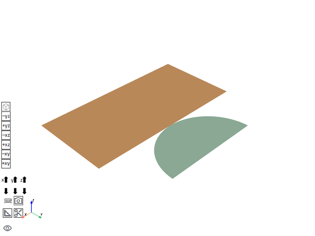
Using a Archard wear model, this example demonstrates contact sliding of a hemispherical ring on a flat ring to produce wear.
The model includes:
Hemispherical ring with a radius of 30 mm made of copper.
Flat ring with an inner radius of 50 mm and an outer radius of 150 mm made of steel.
The hemispherical ring is in contact with the flat ring at the center from the axis of rotation at 100 mm and is subjected to a 1) pressure of 4000 N/mm2 and 2) a rotation with a frequency of 100,000 revolutions/sec.
The application evaluates total deformation and normal stress results, in loading direction, prior to and following wear. In addition, contact pressure prior to wear is evaluated.
Import the necessary libraries#
from pathlib import Path
from typing import TYPE_CHECKING

from PIL import Image
from ansys.mechanical.core import App
from ansys.mechanical.core.examples import delete_downloads, download_file
from matplotlib import image as mpimg
from matplotlib import pyplot as plt
from matplotlib.animation import FuncAnimation

if TYPE_CHECKING:
    import Ansys
    from Ansys.Core.Units import Quantity
    from Ansys.Mechanical.DataModel.Enums import *
Initialize the embedded application#
app = App(globals=globals())
print(app)
Ansys Mechanical [Ansys Mechanical Enterprise]
Product Version:252
Software build date: 06/13/2025 11:25:56
Create functions to set camera and display images#
# Set the path for the output files (images, gifs, mechdat)
output_path = Path.cwd() / "out"


def set_camera_and_display_image(
    camera: Ansys.ACT.Common.Graphics.MechanicalCameraWrapper,
    graphics: Ansys.ACT.Common.Graphics.MechanicalGraphicsWrapper,
    graphics_image_export_settings: Ansys.Mechanical.Graphics.GraphicsImageExportSettings,
    image_output_path: Path,
    image_name: str,
) -> None:
    """Set the camera to fit the model and display the image.

    Parameters
    ----------
    camera : Ansys.ACT.Common.Graphics.MechanicalCameraWrapper
        The camera object to set the view.
    graphics : Ansys.ACT.Common.Graphics.MechanicalGraphicsWrapper
        The graphics object to export the image.
    graphics_image_export_settings : Ansys.Mechanical.Graphics.GraphicsImageExportSettings
        The settings for exporting the image.
    image_output_path : Path
        The path to save the exported image.
    image_name : str
        The name of the exported image file.
    """
    # Set the camera to fit the mesh
    camera.SetFit()
    # Export the mesh image with the specified settings
    image_path = image_output_path / image_name
    graphics.ExportImage(
        str(image_path), image_export_format, graphics_image_export_settings
    )
    # Display the exported mesh image
    display_image(image_path)


def display_image(
    image_path: str,
    pyplot_figsize_coordinates: tuple = (16, 9),
    plot_xticks: list = [],
    plot_yticks: list = [],
    plot_axis: str = "off",
) -> None:
    """Display the image with the specified parameters.

    Parameters
    ----------
    image_path : str
        The path to the image file to display.
    pyplot_figsize_coordinates : tuple
        The size of the figure in inches (width, height).
    plot_xticks : list
        The x-ticks to display on the plot.
    plot_yticks : list
        The y-ticks to display on the plot.
    plot_axis : str
        The axis visibility setting ('on' or 'off').
    """
    # Set the figure size based on the coordinates specified
    plt.figure(figsize=pyplot_figsize_coordinates)
    # Read the image from the file into an array
    plt.imshow(mpimg.imread(image_path))
    # Get or set the current tick locations and labels of the x-axis
    plt.xticks(plot_xticks)
    # Get or set the current tick locations and labels of the y-axis
    plt.yticks(plot_yticks)
    # Turn off the axis
    plt.axis(plot_axis)
    # Display the figure
    plt.show()
Configure graphics for image export#
graphics = app.Graphics
camera = graphics.Camera

# Set the camera orientation to the front view
camera.SetSpecificViewOrientation(ViewOrientationType.Front)

# Set the image export format and settings
image_export_format = GraphicsImageExportFormat.PNG
settings_720p = Ansys.Mechanical.Graphics.GraphicsImageExportSettings()
settings_720p.Resolution = GraphicsResolutionType.EnhancedResolution
settings_720p.Background = GraphicsBackgroundType.White
settings_720p.Width = 1280
settings_720p.Height = 720
settings_720p.CurrentGraphicsDisplay = False

# Rotate the camera on the y-axis
camera.Rotate(180, CameraAxisType.ScreenY)
Download the geometry and material files#
# Download the geometry and material files from the specified paths
geometry_path = download_file("example_07_td43_wear.agdb", "pymechanical", "00_basic")
mat1_path = download_file("example_07_Mat_Copper.xml", "pymechanical", "00_basic")
mat2_path = download_file("example_07_Mat_Steel.xml", "pymechanical", "00_basic")
Import the geometry#
# Define the model
model = app.Model

# Add a geometry import to the geometry import group
geometry_import = model.GeometryImportGroup.AddGeometryImport()

# Set the geometry import settings
geometry_import_format = (
    Ansys.Mechanical.DataModel.Enums.GeometryImportPreference.Format.Automatic
)
geometry_import_preferences = Ansys.ACT.Mechanical.Utilities.GeometryImportPreferences()
geometry_import_preferences.ProcessNamedSelections = True
geometry_import_preferences.ProcessCoordinateSystems = True

# Import the geometry using the specified settings
geometry_import.Import(
    geometry_path, geometry_import_format, geometry_import_preferences
)

# Visualize the model in 3D
app.plot()
[]
Import the materials#
<System.Collections.Generic.List[Material] object at 0x7f3138626300>
Set up the analysis#
# Set up the unit system
app.ExtAPI.Application.ActiveUnitSystem = MechanicalUnitSystem.StandardNMM
Store all main tree nodes as variables
geometry = model.Geometry
coordinate_systems = model.CoordinateSystems
connections = model.Connections
mesh = model.Mesh
named_selections = model.NamedSelections
Add the static structural analysis
model.AddStaticStructuralAnalysis()
static_structural_analysis = model.Analyses[0]

# Store the static structural analysis solution
stat_struct_soln = static_structural_analysis.Solution

# Get the analysis settings for the static structural analysis
analysis_settings: (
    Ansys.ACT.Automation.Mechanical.AnalysisSettings.ANSYSAnalysisSettings
) = static_structural_analysis.Children[0]
Store the named selections as variables
def get_named_selection(name: str):
    """Get the named selection by name."""
    return app.DataModel.GetObjectsByName(name)[0]


curve_named_selection = get_named_selection("curve")
dia_named_selection = get_named_selection("dia")
ver_edge1 = get_named_selection("v1")
ver_edge2 = get_named_selection("v2")
hor_edge1 = get_named_selection("h1")
hor_edge2 = get_named_selection("h2")
all_bodies_named_selection = get_named_selection("all_bodies")
Assign material to the bodies
# Set the model's 2D behavior to axi-symmetric
geometry.Model2DBehavior = Model2DBehavior.AxiSymmetric


def set_material_and_dimension(
    surface_child_index, material, dimension=ShellBodyDimension.Two_D
):
    """Set the material and dimension for a given surface."""
    surface: Ansys.ACT.Automation.Mechanical.Body = geometry.Children[
        surface_child_index
    ].Children[0]
    surface.Material = material
    surface.Dimension = dimension


# Set the material and dimensions for the surface
set_material_and_dimension(0, "Steel")
set_material_and_dimension(1, "Copper")
Configure settings for the contact region
# Add a contact region between the hemispherical ring and the flat ring
contact_region = connections.AddContactRegion()
# Set the source and target locations for the contact region
contact_region.SourceLocation = named_selections.Children[6]
contact_region.TargetLocation = named_selections.Children[3]
# Set contact region properties
contact_region.ContactType = ContactType.Frictionless
contact_region.Behavior = ContactBehavior.Asymmetric
contact_region.ContactFormulation = ContactFormulation.AugmentedLagrange
contact_region.DetectionMethod = ContactDetectionPoint.NodalNormalToTarget
Add a command snippet to use Archard Wear Model
archard_wear_model = """keyo,cid,5,1
keyo,cid,10,2
pi=acos(-1)
slide_velocity=1e5
Uring_offset=100
kcopper=10e-13*slide_velocity*2*pi*Uring_offset
TB,WEAR,cid,,,ARCD
TBFIELD,TIME,0
TBDATA,1,0,1,1,0,0
TBFIELD,TIME,1
TBDATA,1,0,1,1,0,0
TBFIELD,TIME,1.01
TBDATA,1,kcopper,1,1,0,0
TBFIELD,TIME,4
TBDATA,1,kcopper,1,1,0,0"""
cmd1 = contact_region.AddCommandSnippet()
cmd1.AppendText(archard_wear_model)
Insert a remote point
# Add a remote point to the model
remote_point = model.AddRemotePoint()
# Set the remote point location to the center of the hemispherical ring
remote_point.Location = dia_named_selection
remote_point.Behavior = LoadBehavior.Rigid
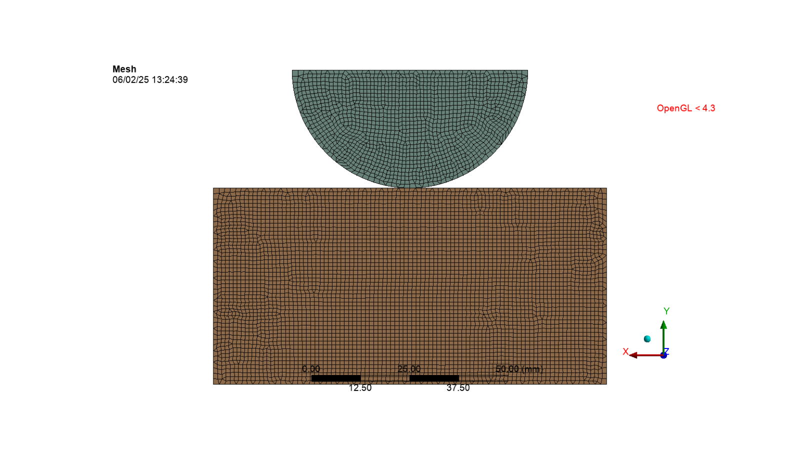
Set properties for the mesh#
# Set the mesh element order and size
mesh.ElementOrder = ElementOrder.Linear
mesh.ElementSize = Quantity("1 [mm]")
Create a function to add edge sizing and properties
def add_edge_sizing_and_properties(
    mesh: Ansys.ACT.Automation.Mechanical.MeshControls.Mesh,
    location,
    divisions,
    sizing_type=SizingType.NumberOfDivisions,
):
    """Set the sizing properties for a given mesh.

    Parameters
    ----------
    mesh : Ansys.Mechanical.DataModel.Mesh
        The mesh object to set the properties for.
    location : Ansys.Mechanical.DataModel.NamedSelection
        The location of the edge to set the sizing for.
    divisions : int
        The number of divisions for the edge.
    sizing_type : SizingType
        The type of sizing to apply (default is NumberOfDivisions).
    """
    edge_sizing = mesh.AddSizing()
    edge_sizing.Location = location
    edge_sizing.Type = sizing_type
    edge_sizing.NumberOfDivisions = divisions
Add edge sizing and properties to the mesh for each named selection
add_edge_sizing_and_properties(mesh, hor_edge1, 70)
add_edge_sizing_and_properties(mesh, hor_edge2, 70)
add_edge_sizing_and_properties(mesh, ver_edge1, 35)
add_edge_sizing_and_properties(mesh, ver_edge2, 35)
add_edge_sizing_and_properties(mesh, dia_named_selection, 40)
add_edge_sizing_and_properties(mesh, curve_named_selection, 60)
Generate the mesh and display the image
mesh.GenerateMesh()
set_camera_and_display_image(camera, graphics, settings_720p, output_path, "mesh.png")
Set the analysis settings#
Create a function to set time steps for the analysis settings
def set_time_steps(initial: str, min: str, max: str) -> None:
    """Set the time step properties for the analysis settings.

    Parameters
    ----------
    initial : str
        The initial time step value.
    min : str
        The minimum time step value.
    max : str
        The maximum time step value.
    """
    analysis_settings.InitialTimeStep = Quantity(initial)
    analysis_settings.MinimumTimeStep = Quantity(min)
    analysis_settings.MaximumTimeStep = Quantity(max)
Set the analysis settings for the static structural analysis
analysis_settings.NumberOfSteps = 2
analysis_settings.CurrentStepNumber = 1
analysis_settings.AutomaticTimeStepping = AutomaticTimeStepping.On
analysis_settings.DefineBy = TimeStepDefineByType.Time
set_time_steps(initial="0.1 [s]", min="0.0001 [s]", max="1 [s]")
analysis_settings.CurrentStepNumber = 2
analysis_settings.Activate()
analysis_settings.StepEndTime = Quantity("4 [s]")
analysis_settings.AutomaticTimeStepping = AutomaticTimeStepping.On
analysis_settings.DefineBy = TimeStepDefineByType.Time
set_time_steps(initial="0.01 [s]", min="0.000001 [s]", max="0.02 [s]")
analysis_settings.LargeDeflection = True
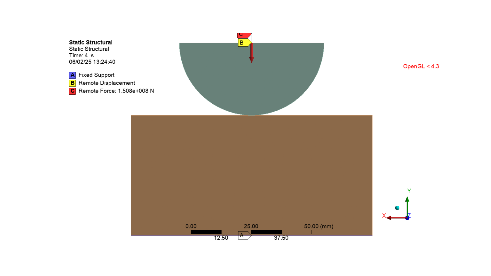
Insert loading and boundary conditions#
# Add a fixed support to the model
fixed_support = static_structural_analysis.AddFixedSupport()
# Set the fixed support location to the first horizontal edge
fixed_support.Location = hor_edge1

# Add a remote displacement to the model
remote_displacement = static_structural_analysis.AddRemoteDisplacement()
# Set the remote displacement location to the remote point
remote_displacement.Location = remote_point
# Add the values for the x-component and rotation about the z-axis
remote_displacement.XComponent.Output.DiscreteValues = [Quantity("0[mm]")]
remote_displacement.RotationZ.Output.DiscreteValues = [Quantity("0[deg]")]

# Add a remote force to the model
remote_force = static_structural_analysis.AddRemoteForce()
# Set the remote force location to the remote point
remote_force.Location = remote_point
# Set the remote force values for the y-component
remote_force.DefineBy = LoadDefineBy.Components
remote_force.YComponent.Output.DiscreteValues = [Quantity("-150796320 [N]")]

#  Nonlinear adaptivity does not support contact criterion yet so a command snippet is used instead
nonlinear_adaptivity = """NLADAPTIVE,all,add,contact,wear,0.50
NLADAPTIVE,all,on,all,all,1,,4
NLADAPTIVE,all,list,all,all"""

# Add the nonlinear adaptivity command snippet to the static structural analysis
cmd2 = static_structural_analysis.AddCommandSnippet()
cmd2.AppendText(nonlinear_adaptivity)
cmd2.StepSelectionMode = SequenceSelectionType.All

# Activate the static structural analysis and display the mesh image
static_structural_analysis.Activate()
set_camera_and_display_image(camera, graphics, settings_720p, output_path, "mesh.png")
Add results to the solution#
def set_properties_for_result(
result: Ansys.ACT.Automation.Mechanical.Results.StressResults.StressResult,
display_time,
orientation_type=NormalOrientationType.YAxis,
display_option=ResultAveragingType.Unaveraged,
):
"""Set the properties for a given result."""
result.NormalOrientation = orientation_type
result.DisplayTime = Quantity(display_time)
result.DisplayOption = display_option
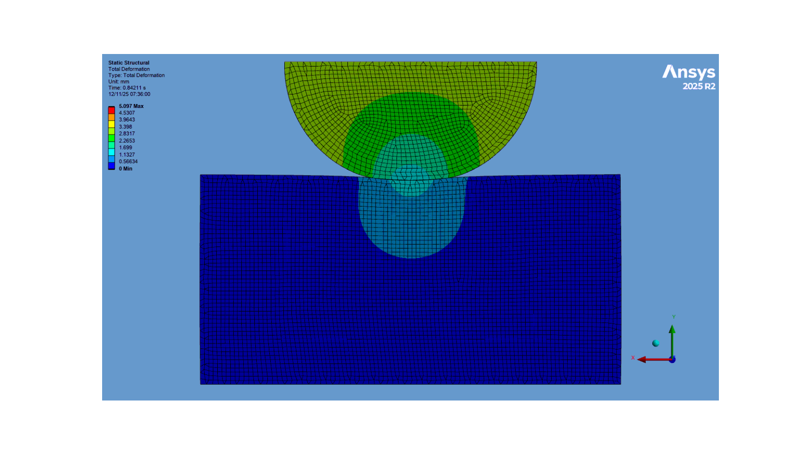
# Add total deformation to the solution
total_deformation = stat_struct_soln.AddTotalDeformation()
# Add normal stress to the solution
normal_stress1 = stat_struct_soln.AddNormalStress()
set_properties_for_result(normal_stress1, display_time="1 [s]")
normal_stress2 = stat_struct_soln.AddNormalStress()
set_properties_for_result(normal_stress1, display_time="4 [s]")
# Add a contact tool to the solution
contact_tool = stat_struct_soln.AddContactTool()
contact_tool.ScopingMethod = GeometryDefineByType.Geometry
# Add selections for the contact tool
selection1 = app.ExtAPI.SelectionManager.AddSelection(all_bodies_named_selection)
selection2 = app.ExtAPI.SelectionManager.CurrentSelection
# Set the contact tool location to the current selection
contact_tool.Location = selection2
# Clear the selection
app.ExtAPI.SelectionManager.ClearSelection()
Add contact pressure to the contact tool
def add_contact_pressure(
    contact_tool: Ansys.ACT.Automation.Mechanical.PostContactTool, display_time
):
    """Add a contact pressure to the contact tool."""
    contact_pressure = contact_tool.AddPressure()
    contact_pressure.DisplayTime = Quantity(display_time)


# Add pressure to the contact tool
add_contact_pressure(contact_tool, display_time="0 [s]")
add_contact_pressure(contact_tool, display_time="4 [s]")
Solve the solution#
stat_struct_soln.Solve(True)
Postprocessing#
Activate the first normal stress result and display the image
app.Tree.Activate([normal_stress1])
set_camera_and_display_image(
    camera, graphics, settings_720p, output_path, "normal_stress.png"
)
Create a function to update the animation frame
def update_animation(frame: int) -> list[mpimg.AxesImage]:
    """Update the animation frame for the GIF.

    Parameters
    ----------
    frame : int
        The frame number to update the animation.

    Returns
    -------
    list[mpimg.AxesImage]
        A list containing the updated image for the animation.
    """
    # Seeks to the given frame in this sequence file
    gif.seek(frame)
    # Set the image array to the current frame of the GIF
    image.set_data(gif.convert("RGBA"))
    # Return the updated image
    return [image]
Display the total deformation animation
# Set the animation export format
animation_export_format = (
    Ansys.Mechanical.DataModel.Enums.GraphicsAnimationExportFormat.GIF
)
# Set the animation export settings
settings_720p = Ansys.Mechanical.Graphics.AnimationExportSettings()
settings_720p.Width = 1280
settings_720p.Height = 720

# Export the animation
total_deformation_gif = output_path / "total_deformation.gif"
total_deformation.ExportAnimation(
    str(total_deformation_gif), animation_export_format, settings_720p
)

# Open the GIF file and create an animation
gif = Image.open(total_deformation_gif)
# Set the subplots for the animation and turn off the axis
figure, axes = plt.subplots(figsize=(16, 9))
axes.axis("off")
# Change the color of the image
image = axes.imshow(gif.convert("RGBA"))

# Create the animation using the figure, update_animation function, and the GIF frames
# Set the interval between frames to 200 milliseconds and repeat the animation
FuncAnimation(
    figure,
    update_animation,
    frames=range(gif.n_frames),
    interval=200,
    repeat=True,
    blit=True,
)

# Show the animation
plt.show()
Print the project tree#
app.print_tree()
├── Project
|  ├── Model
|  |  ├── Geometry Imports (✓)
|  |  |  ├── Geometry Import (✓)
|  |  ├── Geometry (✓)
|  |  |  ├── Steel_Ring
|  |  |  |  ├── Steel_Ring
|  |  |  ├── Hemispherical_Copper_Ring
|  |  |  |  ├── Hemispherical_Copper_Ring
|  |  ├── Materials (✓)
|  |  |  ├── Structural Steel (✓)
|  |  |  ├── Copper (✓)
|  |  |  ├── Steel (✓)
|  |  ├── Coordinate Systems (✓)
|  |  |  ├── Global Coordinate System (✓)
|  |  ├── Remote Points (✓)
|  |  |  ├── Remote Point (✓)
|  |  ├── Connections (✓)
|  |  |  ├── Connection Group (✓)
|  |  |  |  ├── Contact Region (✓)
|  |  |  |  |  ├── Commands (APDL) (✓)
|  |  ├── Mesh (✓)
|  |  |  ├── Edge Sizing (✓)
|  |  |  ├── Edge Sizing 2 (✓)
|  |  |  ├── Edge Sizing 3 (✓)
|  |  |  ├── Edge Sizing 4 (✓)
|  |  |  ├── Edge Sizing 5 (✓)
|  |  |  ├── Edge Sizing 6 (✓)
|  |  ├── Named Selections
|  |  |  ├── all_bodies (✓)
|  |  |  ├── dia (✓)
|  |  |  ├── h1 (✓)
|  |  |  ├── h2 (✓)
|  |  |  ├── v1 (✓)
|  |  |  ├── v2 (✓)
|  |  |  ├── curve (✓)
|  |  ├── Static Structural (✓)
|  |  |  ├── Analysis Settings (✓)
|  |  |  ├── Fixed Support (✓)
|  |  |  ├── Remote Displacement (✓)
|  |  |  ├── Remote Force (✓)
|  |  |  ├── Commands (APDL) (✓)
|  |  |  ├── Solution (✓)
|  |  |  |  ├── Solution Information (✓)
|  |  |  |  ├── Total Deformation (✓)
|  |  |  |  ├── Normal Stress (✓)
|  |  |  |  ├── Normal Stress 2 (✓)
|  |  |  |  ├── Contact Tool (✓)
|  |  |  |  |  ├── Status (✓)
|  |  |  |  |  ├── Pressure (✓)
|  |  |  |  |  ├── Pressure 2 (✓)
Clean up the project#
# Save the project file
mechdat_file = output_path / "contact_wear.mechdat"
app.save(str(mechdat_file))

# Close the app
app.close()

# Delete the downloaded files
delete_downloads()
True
Total running time of the script: (3 minutes 7.198 seconds)