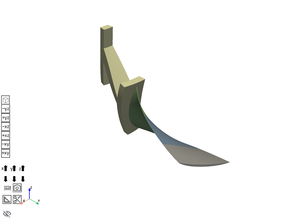
Inverse-Solving analysis of a rotor fan blade with disk

This example demonstrates the inverse-solving analysis of a rotor fan blade with disk. The NASA Rotor 67 fan bladed disk is a subsystem of a turbo fan’s compressor set used in aerospace engine applications. This sector model, representing a challenging industrial example for which the detailed geometry and flow information is available in the public domain, consists of a disk and a fan blade with a sector angle of 16.364 degrees. The sector model represents the running condition or hot geometry of the blade. It is already optimized at the running condition under loading. The primary objective is to obtain the cold geometry (for manufacturing) from the given hot geometry using inverse solving.

• ELEMENTS: SOLID186

• MATERIAL: Elastic Material

• CONTACT: MPC bonded contact pair

To highlight Mechanical APDL inverse-solving technology, this example problem does not involve a cyclic symmetry analysis.

Material Properties:

Temperature	Density	Young’s Modulus	Poisson’s Ratio	Coeff of Thermal Expansion
22 deg C	7840	2.2e11 Pa	0.27	1.2e-5
200 deg C	7740	2e11 Pa	0.28	1.3e-5
300 deg C	7640	1.9e11 Pa	0.29	1.4e-5
600 deg C	7540	1.8e11 Pa	0.30	1.5e-5

Following loads are considered:

The rotational velocity (CGOMGA,0,0,1680) is applied along the global Z axis. The reference temperature is maintained at 22°C, and the temperature loading is applied on the blade (BF)

Expected results:

Inverse-Solving Analysis: A nonlinear static analysis using inverse solving (INVOPT,ON) is performed on the hot geometry of the model to obtain the cold geometry (for manufacturing) and the stress/strain results on the hot geometry.

Import the necessary libraries

from pathlib import Path
from typing import TYPE_CHECKING

from ansys.mechanical.core import App
from ansys.mechanical.core.examples import delete_downloads, download_file
from matplotlib import image as mpimg
from matplotlib import pyplot as plt

if TYPE_CHECKING:
    import Ansys

Initialize the embedded application

app = App(globals=globals())
print(app)

Ansys Mechanical [Ansys Mechanical Enterprise]
Product Version:251
Software build date: 11/27/2024 09:34:44

Create functions to set camera and display images

# Set the path for the output files (images, gifs, mechdat)
output_path = Path.cwd() / "out"


def set_camera_and_display_image(
    camera,
    graphics,
    graphics_image_export_settings,
    image_output_path: Path,
    image_name: str,
) -> None:
    """Set the camera to fit the model and display the image.

    Parameters
    ----------
    camera : Ansys.ACT.Common.Graphics.MechanicalCameraWrapper
        The camera object to set the view.
    graphics : Ansys.ACT.Common.Graphics.MechanicalGraphicsWrapper
        The graphics object to export the image.
    graphics_image_export_settings : Ansys.Mechanical.Graphics.GraphicsImageExportSettings
        The settings for exporting the image.
    image_output_path : Path
        The path to save the exported image.
    image_name : str
        The name of the exported image file.
    """
    # Set the camera to fit the mesh
    camera.SetFit()
    # Export the mesh image with the specified settings
    image_path = image_output_path / image_name
    graphics.ExportImage(
        str(image_path), image_export_format, graphics_image_export_settings
    )
    # Display the exported mesh image
    display_image(image_path)


def display_image(
    image_path: str,
    pyplot_figsize_coordinates: tuple = (16, 9),
    plot_xticks: list = [],
    plot_yticks: list = [],
    plot_axis: str = "off",
) -> None:
    """Display the image with the specified parameters.

    Parameters
    ----------
    image_path : str
        The path to the image file to display.
    pyplot_figsize_coordinates : tuple
        The size of the figure in inches (width, height).
    plot_xticks : list
        The x-ticks to display on the plot.
    plot_yticks : list
        The y-ticks to display on the plot.
    plot_axis : str
        The axis visibility setting ('on' or 'off').
    """
    # Set the figure size based on the coordinates specified
    plt.figure(figsize=pyplot_figsize_coordinates)
    # Read the image from the file into an array
    plt.imshow(mpimg.imread(image_path))
    # Get or set the current tick locations and labels of the x-axis
    plt.xticks(plot_xticks)
    # Get or set the current tick locations and labels of the y-axis
    plt.yticks(plot_yticks)
    # Turn off the axis
    plt.axis(plot_axis)
    # Display the figure
    plt.show()

Download the required files

# Download the geometry file
geometry_path = download_file(
    "example_10_td_055_Rotor_Blade_Geom.pmdb", "pymechanical", "embedding"
)

# Download the material file
mat_path = download_file(
    "example_10_td_055_Rotor_Blade_Mat_File.xml", "pymechanical", "embedding"
)

# Download the CFX pressure data
cfx_data_path = download_file(
    "example_10_CFX_ExportResults_FT_10P_EO2.csv", "pymechanical", "embedding"
)

# Download the temperature data file
temp_data_path = download_file(
    "example_10_Temperature_Data.txt", "pymechanical", "embedding"
)

Configure graphics for image export

# Define the graphics and camera
graphics = app.Graphics
camera = graphics.Camera

# Set the camera orientation to the isometric view and set the camera to fit the model
camera.SetSpecificViewOrientation(ViewOrientationType.Iso)
camera.SetFit()

# Set the image export format and settings
image_export_format = GraphicsImageExportFormat.PNG
settings_720p = Ansys.Mechanical.Graphics.GraphicsImageExportSettings()
settings_720p.Resolution = (
    Ansys.Mechanical.DataModel.Enums.GraphicsResolutionType.EnhancedResolution
)
settings_720p.Background = Ansys.Mechanical.DataModel.Enums.GraphicsBackgroundType.White
settings_720p.Width = 1280
settings_720p.Height = 720
settings_720p.CurrentGraphicsDisplay = False

Import the geometry

# Define the model
model = app.Model

# Add the geometry import to the geometry import group
geometry_import_group = model.GeometryImportGroup
geometry_import = geometry_import_group.AddGeometryImport()

# Set the geometry import format and settings
geometry_import_format = (
    Ansys.Mechanical.DataModel.Enums.GeometryImportPreference.Format.Automatic
)
geometry_import_preferences = Ansys.ACT.Mechanical.Utilities.GeometryImportPreferences()
geometry_import_preferences.ProcessNamedSelections = True
geometry_import_preferences.NamedSelectionKey = ""
geometry_import_preferences.ProcessMaterialProperties = True
geometry_import_preferences.ProcessCoordinateSystems = True

# Import the geometry with the specified settings
geometry_import.Import(
    geometry_path, geometry_import_format, geometry_import_preferences
)

# Visualize the model in 3D
app.plot()

Static Scene

Interactive Scene

Assign materials

Import material from the xml file and assign it to bodies

# Define and import the materials
materials = model.Materials
materials.Import(mat_path)

# Assign the imported material to the components
part1 = app.DataModel.GetObjectsByName(r"Component2\Rotor11")[0]
part2 = app.DataModel.GetObjectsByName("Component3")[0]
part2_blade1 = part2.Children[0]
part2_blade2 = part2.Children[1]
part2_blade3 = part2.Children[2]
part1.Material = "MAT1 (Setup, File1)"
part2_blade1.Material = "MAT1 (Setup, File1)"
part2_blade2.Material = "MAT1 (Setup, File1)"
part2_blade3.Material = "MAT1 (Setup, File1)"

Define the unit system and store variables

# Select MKS units
app.ExtAPI.Application.ActiveUnitSystem = MechanicalUnitSystem.StandardMKS

# Store all main tree nodes as variables
geometry = model.Geometry
mesh = model.Mesh
materials = model.Materials
coordinate_systems = model.CoordinateSystems
named_selections = model.NamedSelections

Define the named selections

Create a function to get named selections by name

def get_named_selection(ns_list: list) -> dict:
    """Get the named selection by name.

    Parameters
    ----------
    ns_list : list
        A list of named selection names to retrieve.

    Returns
    -------
    dict
        A dictionary containing the named selection objects.
    """
    ns_dict = {}
    for name in ns_list:
        ns_dict[name] = app.DataModel.GetObjectsByName(name)[0]
    return ns_dict

Create a dictionary of named selections

named_selections_names = [
    "Blade",
    "Blade_Surf",
    "Fix_Support",
    "Blade_Hub",
    "Hub_Contact",
    "Blade_Target",
    "Hub_Low",
    "Hub_High",
    "Blade1",
    "Blade1_Source",
    "Blade1_Target",
    "Blade2",
    "Blade2_Source",
    "Blade2_Target",
    "Blade3",
    "Blade3_Source",
    "Blade3_Target",
]
ns_dict = get_named_selection(named_selections_names)

Add a coordinate system

coordinate_systems = model.CoordinateSystems
coord_system = coordinate_systems.AddCoordinateSystem()
# Create cylindrical coordinate system
coord_system.CoordinateSystemType = (
    Ansys.ACT.Interfaces.Analysis.CoordinateSystemTypeEnum.Cylindrical
)
coord_system.OriginDefineBy = CoordinateSystemAlignmentType.Component
coord_system.OriginDefineBy = CoordinateSystemAlignmentType.Fixed

Add contact regions

connections = model.Connections
contact_region1 = connections.AddContactRegion()
contact_region1.SourceLocation = named_selections.Children[6]
contact_region1.TargetLocation = named_selections.Children[5]
contact_region1.Behavior = ContactBehavior.AutoAsymmetric
contact_region1.ContactFormulation = ContactFormulation.MPC

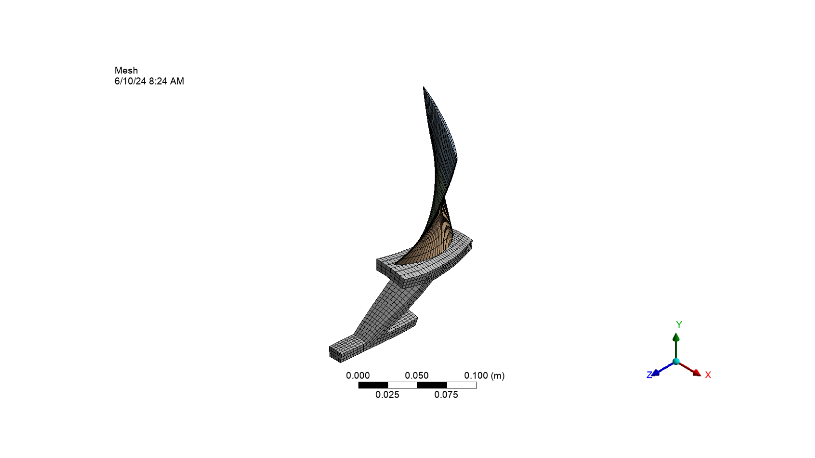
Define the mesh settings and generate the mesh

Set the mesh settings

mesh = model.Mesh

# Set the mesh settings
mesh.ElementSize = Quantity(0.004, "m")
mesh.UseAdaptiveSizing = False
mesh.MaximumSize = Quantity(0.004, "m")
mesh.ShapeChecking = 0

Create a function to add an automatic method to the mesh

def add_automatic_method(
    mesh,
    location_index: int,
    source_loc_index: int = None,
    target_loc_index: int = None,
    method=MethodType.Sweep,
    source_target_selection=2,
    sweep_number_divisions=5,
    set_src_target_properties: bool = True,
):
    """Add an automatic method to the mesh."""
    automatic_method = mesh.AddAutomaticMethod()
    automatic_method.Location = named_selections.Children[location_index]
    automatic_method.Method = method
    if set_src_target_properties:
        automatic_method.SourceTargetSelection = source_target_selection
        if source_loc_index:
            automatic_method.SourceLocation = named_selections.Children[
                source_loc_index
            ]
        if target_loc_index:
            automatic_method.TargetLocation = named_selections.Children[
                target_loc_index
            ]
    automatic_method.SweepNumberDivisions = sweep_number_divisions


# Add an automatic method for the hub
add_automatic_method(
    mesh, location_index=0, sweep_number_divisions=6, set_src_target_properties=False
)

Add match control and sizing to the mesh

# Add match control to the mesh
match_control_hub = mesh.AddMatchControl()
# Set the low and high named selections to named selections' children at indices 7 and 8
match_control_hub.LowNamedSelection = named_selections.Children[7]
match_control_hub.HighNamedSelection = named_selections.Children[8]
# Set the rotation axis to the second child of the coordinate systems
match_control_hub.RotationAxis = coordinate_systems.Children[1]

# Add sizing to the mesh
sizing_blade = mesh.AddSizing()
# Set properties for the sizing blade
sizing_blade.Location = named_selections.Children[5]
sizing_blade.ElementSize = Quantity(1e-2, "m")
sizing_blade.CaptureCurvature = True
sizing_blade.CurvatureNormalAngle = Quantity(0.31, "rad")
sizing_blade.LocalMinimumSize = Quantity(0.0005, "m")

Add automatic methods for each blad

add_automatic_method(mesh, 9, 10, 11)
add_automatic_method(mesh, 12, 13, 14)
add_automatic_method(mesh, 15, 16, 17)

Generate the mesh and display the image

mesh.GenerateMesh()
set_camera_and_display_image(
    camera, graphics, settings_720p, output_path, "blade_mesh.png"
)

Define the analysis settings

# Add a static structural analysis to the model
model.AddStaticStructuralAnalysis()
static_structural_analysis = model.Analyses[0]

# Set the analysis settings
analysis_settings = app.ExtAPI.DataModel.Project.Model.Analyses[0].AnalysisSettings
analysis_settings.AutomaticTimeStepping = AutomaticTimeStepping.On
analysis_settings.NumberOfSubSteps = 10

# Activate the analysis settings
analysis_settings.Activate()

# Add a command snippet to the static structural analysis with the archard wear model
cmd1 = static_structural_analysis.AddCommandSnippet()
# Add convergence criterion using command snippet.
archard_wear_model = """CNVTOL,U,1.0,5e-5,1,,"""
cmd1.AppendText(archard_wear_model)

# Set the analysis settings for inverse solving
analysis_settings.InverseOption = True
analysis_settings.LargeDeflection = True

Define the boundary conditions

# Add rotational velocity to the static structural analysis
rotational_velocity = static_structural_analysis.AddRotationalVelocity()
rotational_velocity.DefineBy = LoadDefineBy.Components
# Set z-component input values for the rotational velocity
rotational_velocity.ZComponent.Inputs[0].DiscreteValues = [
    Quantity("0 [s]"),
    Quantity("1 [s]"),
    Quantity("2 [s]"),
]
# Set z-component output values for the rotational velocity
rotational_velocity.ZComponent.Output.DiscreteValues = [
    Quantity("0 [rad/s]"),
    Quantity("1680 [rad/s]"),
    Quantity("1680 [rad/s]"),
]

# Add a fixed support to the static structural analysis
fixed_support = static_structural_analysis.AddFixedSupport()
# Set the fixed support location to the named selection at index 3
fixed_support.Location = named_selections.Children[3]

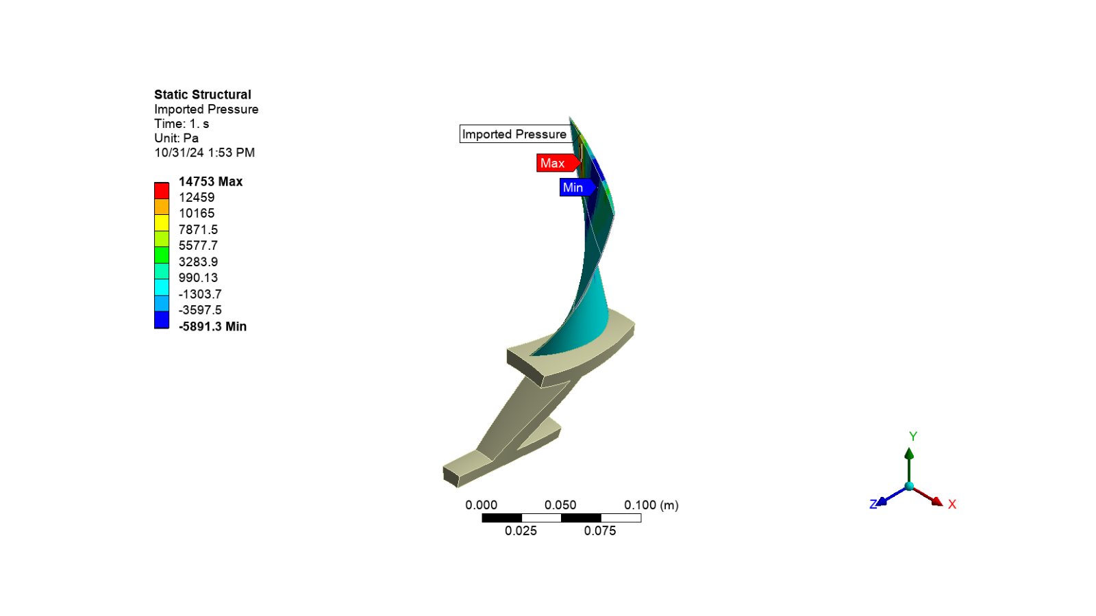
Import and apply temperature and CFX pressure to the structural blade & its surface

Create a function to process the CFX pressure and temperature data files

def process_external_data(
    external_data_path: str,
    skip_rows: int,
    skip_footer: int,
    data_type: str,
    location_index: int,
):
    """Process the external data file and set its properties."""
    # Add imported load external data to the static structural analysis
    imported_load_group = static_structural_analysis.AddImportedLoadExternalData()

    external_data_files = Ansys.Mechanical.ExternalData.ExternalDataFileCollection()
    external_data_files.SaveFilesWithProject = False
    file = Ansys.Mechanical.ExternalData.ExternalDataFile()
    external_data_files.Add(file)

    file.Identifier = "File1"
    file.Description = ""
    file.IsMainFile = False
    file.FilePath = external_data_path
    # Set the file format to delimited
    file.ImportSettings = Ansys.Mechanical.ExternalData.ImportSettingsFactory.GetSettingsForFormat(
        Ansys.Mechanical.DataModel.MechanicalEnums.ExternalData.ImportFormat.Delimited
    )

    # Set up import settings for the external data file
    import_settings = file.ImportSettings
    import_settings.SkipRows = skip_rows
    import_settings.SkipFooter = skip_footer
    import_settings.Delimiter = ","
    import_settings.AverageCornerNodesToMidsideNodes = False
    import_settings.UseColumn(
        0,
        Ansys.Mechanical.DataModel.MechanicalEnums.ExternalData.VariableType.XCoordinate,
        "m",
        "X Coordinate@A",
    )
    import_settings.UseColumn(
        1,
        Ansys.Mechanical.DataModel.MechanicalEnums.ExternalData.VariableType.YCoordinate,
        "m",
        "Y Coordinate@B",
    )
    import_settings.UseColumn(
        2,
        Ansys.Mechanical.DataModel.MechanicalEnums.ExternalData.VariableType.ZCoordinate,
        "m",
        "Z Coordinate@C",
    )
    if data_type == "pressure":
        import_settings.UseColumn(
            3,
            Ansys.Mechanical.DataModel.MechanicalEnums.ExternalData.VariableType.Pressure,
            "Pa",
            "Pressure@D",
        )
    elif data_type == "temperature":
        import_settings.UseColumn(
            3,
            Ansys.Mechanical.DataModel.MechanicalEnums.ExternalData.VariableType.Temperature,
            "C",
            "Temperature@D",
        )
    # Import external data files to the imported load group
    imported_load_group.ImportExternalDataFiles(external_data_files)
    if data_type == "pressure":
        # Add imported pressure to the imported load group
        added_obj = imported_load_group.AddImportedPressure()
    elif data_type == "temperature":
        # Add imported body temperature to the imported load group
        added_obj = imported_load_group.AddImportedBodyTemperature()
    # Set properties for the imported pressure
    added_obj.Location = named_selections.Children[location_index]
    if data_type == "pressure":
        added_obj.AppliedBy = LoadAppliedBy.Direct
    added_obj.ImportLoad()

    return added_obj

Import and apply CFX pressure to the structural blade surface

pressure = process_external_data(
    cfx_data_path, skip_rows=17, skip_footer=0, data_type="pressure", location_index=2
)

# Activate the imported pressure or temperature and display the image
app.Tree.Activate([pressure])
set_camera_and_display_image(
    camera, graphics, settings_720p, output_path, f"imported_pressure.png"
)

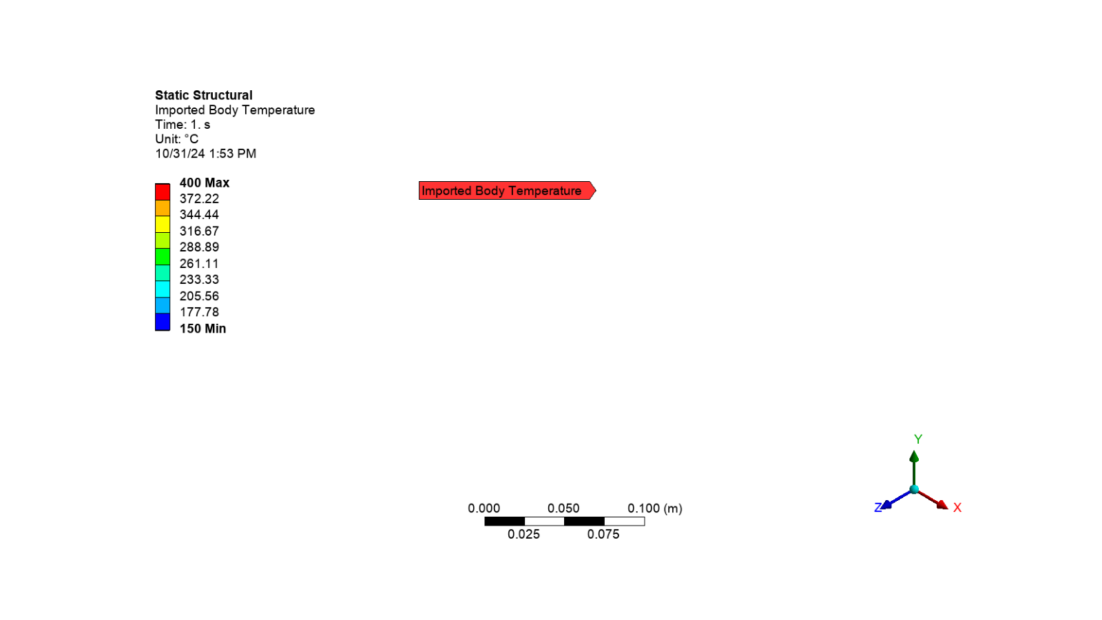
Import and apply temperature to the structural blade

temperature = process_external_data(
    temp_data_path,
    skip_rows=0,
    skip_footer=0,
    data_type="temperature",
    location_index=1,
)

# Activate the imported temperature and display the image
app.Tree.Activate([temperature])
set_camera_and_display_image(
    camera, graphics, settings_720p, output_path, f"imported_temperature.png"
)

Add results to the solution

# Define the static structural analysis solution
solution = static_structural_analysis.Solution

# Add total deformation results to the solution
total_deformation1 = solution.AddTotalDeformation()
total_deformation1.DisplayTime = Quantity("1 [s]")

# Add equivalent stress results to the solution
equivalent_stress1 = solution.AddEquivalentStress()
equivalent_stress1.DisplayTime = Quantity("1 [s]")

# Add equivalent total strain results to the solution
equivalent_total_strain1 = solution.AddEquivalentTotalStrain()
equivalent_total_strain1.DisplayTime = Quantity("1 [s]")

# Add thermal strain results to the solution
thermal_strain1 = solution.AddThermalStrain()
thermal_strain1.DisplayTime = Quantity("1 [s]")

Solve the solution

# Solve the inverse analysis on the blade model
solution.Solve(True)
soln_status = solution.Status

Postprocessing

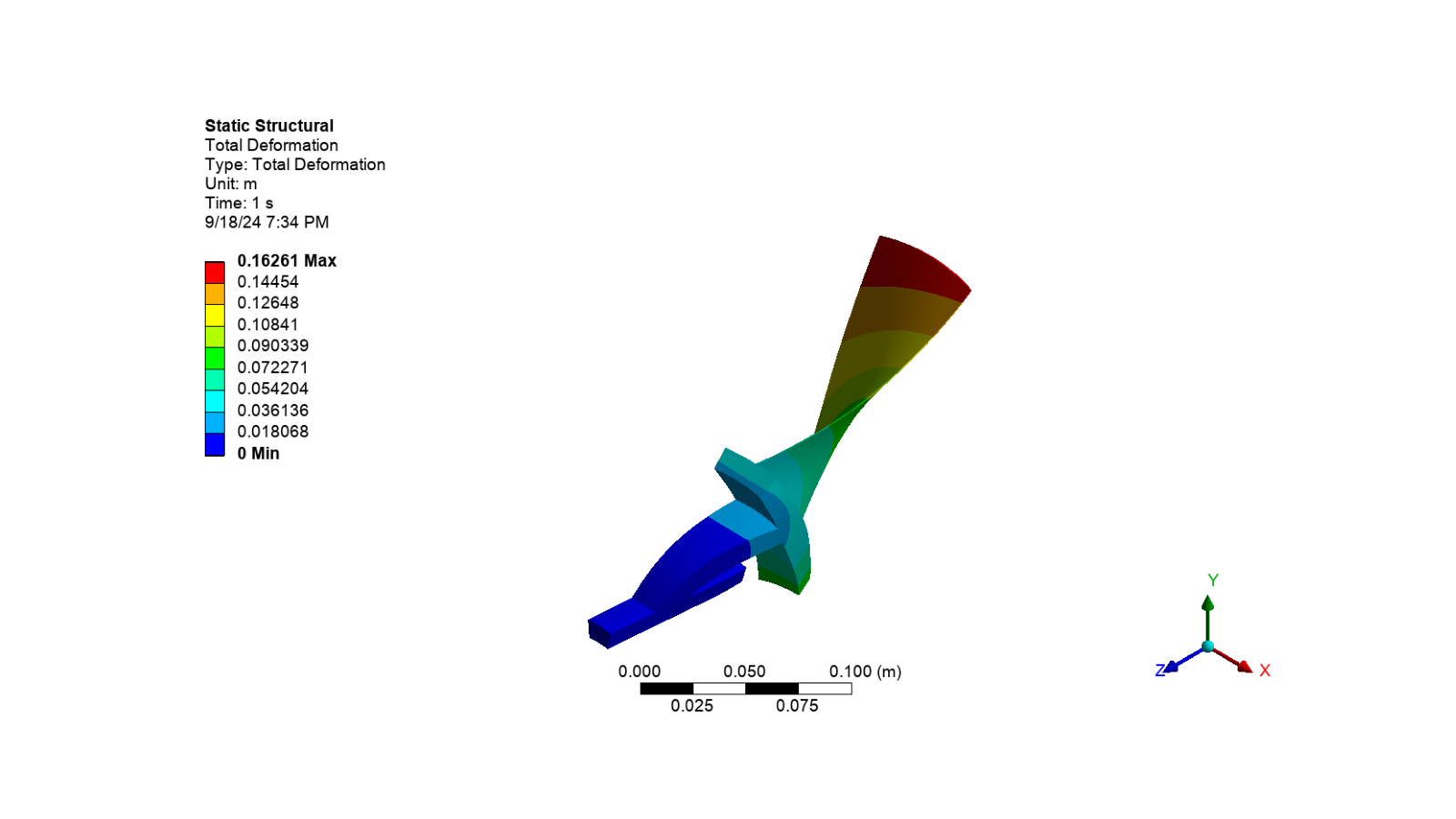
Display the total deformation image

# Activate the total deformation results
app.Tree.Activate([total_deformation1])
# Set the extra model display to no wireframe
graphics.ViewOptions.ResultPreference.ExtraModelDisplay = (
    Ansys.Mechanical.DataModel.MechanicalEnums.Graphics.ExtraModelDisplay.NoWireframe
)
# Set the camera to fit the model and export the image
set_camera_and_display_image(
    camera, graphics, settings_720p, output_path, "total_deformation.png"
)

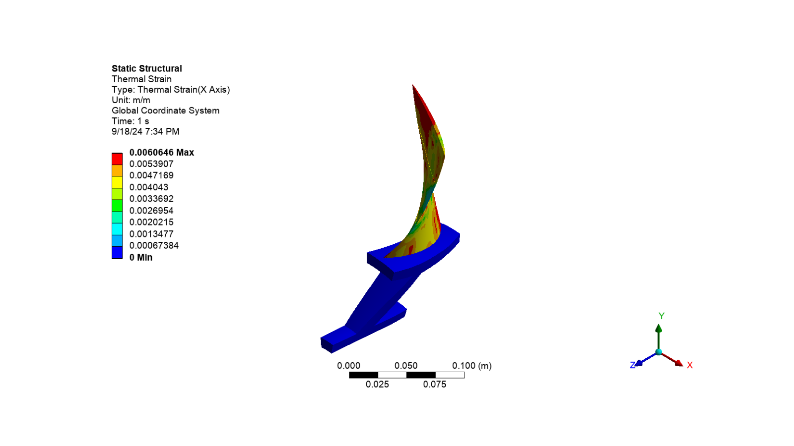
Display the thermal strain image

# Activate the thermal strain results
app.Tree.Activate([thermal_strain1])
# Set the camera to fit the model and export the image
set_camera_and_display_image(
    camera, graphics, settings_720p, output_path, "thermal_strain.png"
)

Clean up the project

# Save the project
mechdat_file = output_path / "blade_inverse.mechdat"
app.save(str(mechdat_file))

# Close the app
app.close()

# Delete the example file
delete_downloads()

True